
Author: Gerd Doeben-Henisch
Changelog: Febr 9, 2025 – Febr 9, 2025
Email: info@uffmm.org
TRANSLATION: The following text is a translation from a German version into English. For the translation I am using the software @chatGPT4o with manual modifications.
CONTENT TREE
This text is part of the TOPIC Philosophy of Science.
CONTEXT
This is a direct continuation of the preceding texts
- “WHAT IS LIFE? WHAT ROLE DO WE PLAY? IST THERE A FUTURE?”
- “WHAT IS LIFE? … DEMOCRACY – CITIZENS”
- WHAT IS LIFE? … PHILOSOPHY OF LIFE
INTRODUCTION
In the preceding texts, the ‘framework’ has been outlined within which the following texts on the topic “What is life? …” will unfold. A special position is taken by the text on ‘philosophy,’ as it highlights the ‘perspective’ in which we find ourselves when we begin to think about ourselves and the surrounding world—and then also to ‘write’ about it. As a reminder of the philosophical perspective, here is the last section as a quote:
“Ultimately, ‘philosophy’ is a ‘total phenomenon’ that manifests itself in the interplay of many people in everyday life, is experienceable, and can only take shape here, in process form. ‘Truth,’ as the ‘hard core’ of any reality-related thinking, can therefore always be found only as a ‘part’ of a process in which the active interconnections significantly contribute to the ‘truth of a matter.’ Truth is therefore never ‘self-evident,’ never ‘simple,’ never ‘free of cost’; truth is a ‘precious substance’ that requires every effort to be ‘gained,’ and its state is a ‘fleeting’ one, as the ‘world’ within which truth can be ‘worked out’ continuously changes as a world. A major factor in this constant change is life itself: the ‘existence of life’ is only possible within an ‘ongoing process’ in which ‘energy’ can make ‘emergent images’ appear—images that are not created for ‘rest’ but for a ‘becoming,’ whose ultimate goal still appears in many ways ‘open’: Life can indeed—partially—destroy itself or—partially—empower itself. Somewhere in the midst of this, we find ourselves. The current year ‘2025’ is actually of little significance in this regard.”
WHAT IS LIFE? … If life is ‘More,’ ‘much more’ …
In the first text of this project, “What is Life,” much has already been said under the label ‘EARTH@WORK. Cradle of Humankind’—in principle, everything that can and must be said about a ‘new perspective’ on the ‘phenomenon of life’ in light of modern scientific and philosophical insights. As a reminder, here is the text:
“The existence [of planet Earth] was in fact the prerequisite for biological life as we know it today to have developed the way we have come to understand it. Only in recent years have we begun to grasp how the known ‘biological life’ (Nature 2) could have ‘evolved’ from ‘non-biological life’ (Nature 1). Upon deeper analysis, one can recognize not only the ‘commonality’ in the material used but also the ‘novel extensions’ that distinguish the ‘biological’ from the ‘non-biological.’ Instead of turning this ‘novelty’ into an opposition, as human thought has traditionally done (e.g., ‘matter’ versus ‘spirit,’ ‘matter’ versus ‘mind’), one can also understand it as a ‘manifestation’ of something ‘more fundamental,’ as an ‘emergence’ of new properties that, in turn, point to characteristics inherent in the ‘foundation of everything’—namely, in ‘energy’—which only become apparent when increasingly complex structures are formed. This novel interpretation is inspired by findings from modern physics, particularly quantum physics in conjunction with astrophysics. All of this suggests that Einstein’s classical equation (1905) e=mc² should be interpreted more broadly than has been customary so far (abbreviated: Plus(e=mc²)).”
This brief text will now be further expanded to make more visible the drama hinted at by the convergence of many new insights. Some may find these perspectives ‘threatening,’ while others may see them as the ‘long-awaited liberation’ from ‘false images’ that have so far rather ‘obscured’ our real possible future.
Different Contexts
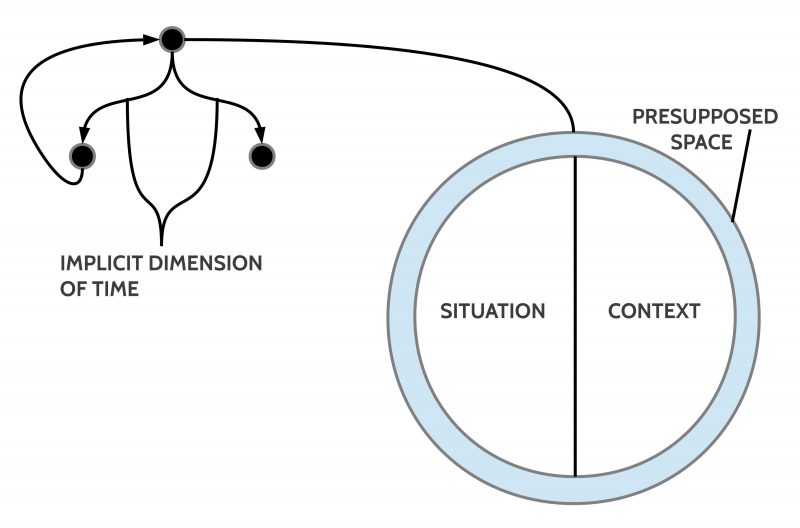
If we see an ‘apple’ in isolation, this apple, with its shapes and colors, appears somehow ‘indeterminate’ by itself. But if we ‘experience’ that an apple can be ‘eaten,’ taste it, feel its effect on our body, then the apple becomes ‘part of a context.’ And if we also happen to ‘know’ something about its composition and its possible effects on our body, then the ‘image of experience’ expands into an ‘image of knowledge,’ forming a ‘context of experience and knowledge’ within us—one that pulls the apple out of its ‘initial indeterminacy.’ As part of such a context, the apple is ‘more’ than before.
The same applies to a ‘chair’: on its own, it has a shape, colors, and surface characteristics, but nothing more. If we experience that this chair is placed in a ‘room’ along with other ‘pieces of furniture,’ that we can ‘sit on a chair,’ that we can move it within the room, then an experienced image of a larger whole emerges—one in which the chair is a part with specific properties that distinguish it from other pieces of furniture. If we then also know that furniture appears in ‘rooms,’ which are parts of ‘houses,’ another rather complex ‘context of experience and knowledge’ forms within us—again making the individual chair ‘more’ than before.
We can apply this kind of thinking to many objects in everyday life. In fact, there is no single object that exists entirely on its own. This is particularly evident in ‘biological objects’ such as animals, plants, and insects.
Let’s take ourselves—humans—as an example. If we let our gaze wander from the spot where each of us is right now, across the entire country, the whole continent, even the entire sphere of our planet, we find that today (2025), humans are almost everywhere. In the standard form of men and women, there is hardly an environment where humans do not live. These environments can be very simple or densely packed with towering buildings, machines, and people in tight spaces. Once we broaden our perspective like this, it becomes clear that we humans are also ‘part of something’: both of the geographical environment we inhabit and of a vast biological community.
In everyday life, we usually only encounter a few others—sometimes a few hundred, in special cases even a few thousand—but through available knowledge, we can infer that we are billions. Again, it is the ‘context of experience and knowledge’ that places us in a larger framework, in which we are clearly ‘part of something greater.’ Here, too, the context represents something ‘more’ compared to ourselves as an individual person, as a single citizen, as a lone human being.
Time, Time Slices, …
If we can experience and think about the things around us—including ourselves—within the ‘format’ of ‘contexts,’ then it is only a small step to noticing the phenomenon of ‘change.’ In the place where we are right now, in the ‘now,’ in the ‘present moment,’ there is no change; everything is as it is. But as soon as the ‘current moment’ is followed by a ‘new moment,’ and then more and more new moments come ‘one after another,’ we inevitably begin to notice ‘changes’: things change, everything in this world changes; there is nothing that does not change!
In ‘individual experience,’ it may happen that, for several moments, we do not ‘perceive anything’ with our eyes, ears, sense of smell, or other senses. This is possible because our body’s sensory organs perceive the world only very roughly. However, with the methods of modern science, which can look ‘infinitely small’ and ‘infinitely large,’ we ‘know’ that, for example, our approximately 37 trillion (10¹²) body cells are highly active at every moment—exchanging ‘messages,’ ‘materials,’ repairing themselves, replacing dead cells with new ones, and so on. Thus, our own body is exposed to a veritable ‘storm of change’ at every moment without us being able to perceive it. The same applies to the realm of ‘microbes,’ the smallest living organisms that we cannot see, yet exist by the billions—not only ‘around us’ but also colonizing our skin and remaining in constant activity. Additionally, the materials that make up the buildings around us are constantly undergoing transformation. Over the years, these materials ‘age’ to the point where they can no longer fulfill their intended function; bridges, for example, can collapse—as we have unfortunately witnessed.
In general, we can only speak of ‘change’ if we can distinguish a ‘before’ and an ‘after’ and compare the many properties of a ‘moment before’ with those of a ‘moment after.’ In the realm of our ‘sensory perception,’ there is always only a ‘now’—no ‘before’ and ‘after.’ However, through the function of ‘memory’ working together with the ability to ‘store’ current events, our ‘brain’ possesses the remarkable ability to ‘quasi-store’ moments to a certain extent. Additionally, it can compare ‘various stored moments’ with a current sensory perception based on specific criteria. If there are ‘differences’ between the ‘current sensory perception’ and the previously ‘stored moments,’ our brain ‘notifies us’—we ‘notice’ the change.
This phenomenon of ‘perceived change’ forms the basis for our ‘experience of time.’ Humans have always relied on ‘external events’ to help categorize perceived changes within a broader framework (day-night cycles, seasons, various star constellations, timekeeping devices like various ‘clocks’ … supported by time records and, later, calendars). However, the ability to experience change remains fundamental to us.
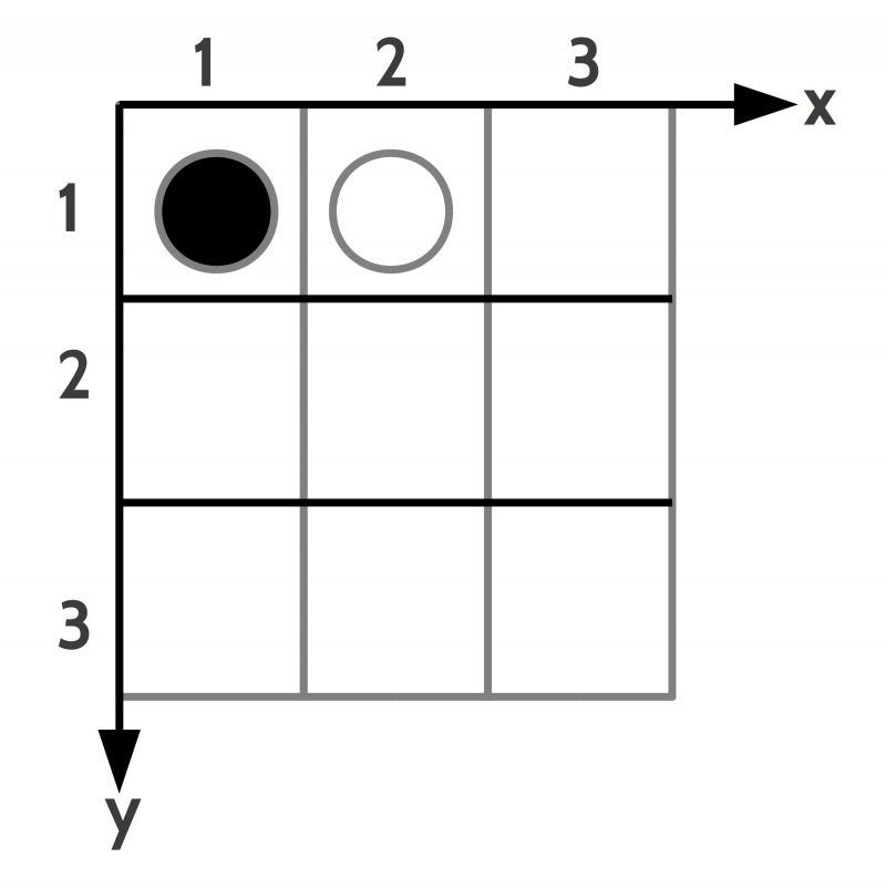
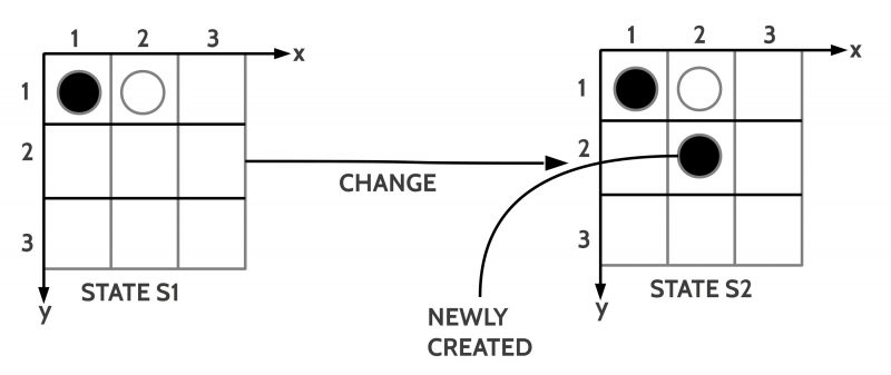
Reflecting on all of this, one can formulate the concept of a ‘time slice’: If we imagine a ‘time segment’—which can be of any length (nanoseconds, seconds, hours, years, …)—and consider all locations on our planet, along with everything present in those locations, as a single ‘state,’ then repeating this process for each subsequent time segment creates a ‘sequence’ or ‘series’ of ‘time slices.’ Within this framework, every change occurring anywhere within a state manifests with its ‘effects’ in one of the following time slices. Depending on the ‘thickness of the time slice,’ these effects appear in the ‘immediately following slice’ or much later. In this model, nothing is lost. Depending on its ‘granularity,’ the model can be ‘highly precise’ or ‘very coarse.’ For instance, population statistics in a German municipality are only recorded once a year, on the last day of the year. If this data were collected weekly, the individual parameters (births, deaths, immigration, emigration, …) would vary significantly.
In the transition from one time slice to the next, every change has an impact—including everything that every individual person does. However, we must distinguish between immediate effects (e.g., a young person attending school regularly) and ‘long-term outcomes’ (e.g., a school diploma, acquired competencies, …), which do not manifest as direct, observable change events. The acquisition of experiences, knowledge, and skills affects the ‘inner structure’ of a person by building ‘various cognitive structures’ that enable the individual to ‘plan, decide, and act’ in new ways. This internal ‘structural development’ of a person is not directly observable, yet it can significantly influence the ‘quality of behavior.’
Time Slices of Life on Planet Earth
It was already mentioned that the ‘thickness of a time slice’ affects which events can be observed. This is related to the fact that we have come to know many ‘different types of change’ on planet Earth. Processes in the sky and in nature generally seem to take ‘longer,’ whereas the effects of specific mechanical actions occur rather ‘quickly,’ and changes to the Earth’s surface take thousands, many thousands, or even millions of years.
Here, the focus is on the major developmental steps of (biological) life on planet Earth. We ourselves—as Homo sapiens—are part of this development, and it may be interesting to explore whether our ‘participation in the great web of life’ reveals perspectives that we cannot practically perceive in the ‘everyday life’ of an individual, even though these perspectives might be of great significance to each of us.
The selection of ‘key events’ in the development of life on Earth naturally depends heavily on the ‘prior knowledge’ with which one approaches the task. Here, I have selected only those points that are found in nearly all major publications. The given time points, ‘from which’ these events are recognized, are inherently ‘imprecise,’ as both the ‘complexity’ of the events and the challenges of ‘temporal determination’ prevent greater accuracy even today. The following key events have been selected:
- Molecular Evolution (from ~3.9 billion years ago)
- Prokaryotic Cells (from ~3.5 billion years ago)
- Great Oxygenation Event (from ~2.5 billion years ago)
- Eukaryotic Cells (from ~1.5 billion years ago)
- Multicellular Life (from ~600 million years ago)
- Emergence of the Homo Genus (from ~2.5 million years ago)
- Emergence of Homo sapiens (from ~300,000 years ago)
- Emergence of Artificial Intelligence (from ~21st century)
I was then interested in calculating the time gaps between these events. For this calculation, only the starting points of the key events were used, as no precise date can be reliably determined for their later progression. The following table was derived:
- Molecular Evolution to Prokaryotic Cells: 400 million years
- Prokaryotic Cells to the Great Oxygenation Event: 1 billion years
- Great Oxygenation Event to Eukaryotic Cells: 1 billion years
- Eukaryotic Cells to Multicellular Life: 900 million years
- Multicellular Life to the Emergence of the Homo Genus: 597.5 million years
- Homo Genus to Homo sapiens: 2.2 million years
- Homo sapiens to Artificial Intelligence: 297,900 years
Next, I converted these time intervals into ‘percentage shares of the total time’ of 3.9 billion years. This resulted in the following table:
- Molecular Evolution to Prokaryotic Cells: 400 million years = 10.26%
- Prokaryotic Cells to the Great Oxygenation Event: 1 billion years = 25.64%
- Great Oxygenation Event to Eukaryotic Cells: 1 billion years = 25.64%
- Eukaryotic Cells to Multicellular Life: 900 million years = 23.08%
- Multicellular Life to the Emergence of the Homo Genus: 597.5 million years = 15.32%
- Homo Genus to Homo sapiens: 2.2 million years = 0.056%
- Homo sapiens to Artificial Intelligence: 297,900 years = 0.0076%
With these numbers, one can examine whether these data points on a timeline reveal any notable characteristics. Of course, purely mathematically, there are many options for what to look for. My initial interest was simply to determine whether there could be a mathematically defined curve that significantly correlates with these data points.
After numerous tests with different estimation functions (see explanations in the appendix), the logistic (S-curve) function emerged as the one that, by its design, best represents the dynamics of the real data regarding the development of biological systems.

For this estimation function, the data points “Molecular Evolution” and “Emergence of AI” were excluded, as they do not directly belong to the development of biological systems in the narrower sense. This resulted in the following data points as the basis for finding an estimation function:
0  Molecular Evolution to Prokaryotes          4.000000e+08 (NOT INCLUDED)
1  Prokaryotes to Great Oxygenation Event      1.000000e+09
2  Oxygenation Event to Eukaryotes             1.000000e+09
3  Eukaryotes to Multicellular Organisms       9.000000e+08
4  Multicellular Organisms to Homo             5.975000e+08
5  Homo to Homo sapiens                        2.200000e+06
6  Homo sapiens to AI                          2.979000e+05 (NOT INCLUDED)
For the selected events, the corresponding cumulative time values were:
0  0.400000
1  1.400000
2  2.400000
3  3.300000
4  3.897500
5  3.899700
6  3.899998
Based on these values, the prediction for the next “significant” event in the development of biological systems resulted in a time of 4.0468 billion years (our present is at 3.899998 billion years). This means that, under a conservative estimate, the next structural event is expected to occur in approximately 146.8 million years. However, it is also not entirely unlikely that it could happen in about 100 million years instead.
The curve reflects the “historical process” that classical biological systems have produced up to Homo sapiens using their previous means. However, with the emergence of the Homo genus—and especially with the life form Homo sapiens—completely new properties come into play. Within the subpopulation of Homo sapiens, there exists a life form that, through its cognitive dimension and new symbolic communication, can generate much faster and more complex foundations for action.
Thus, it cannot be ruled out that the next significant evolutionary event might occur well before 148 million years or even before 100 million years.
This working hypothesis is further reinforced by the fact that Homo sapiens, after approximately 300,000 years, has now developed machines that can be programmed. These machines can already provide substantial assistance in tasks that exceed the cognitive processing capacity of an individual human brain in navigating our complex world.
Although machines, as non-biological systems, lack an intrinsic developmental basis like biological systems, in the format of co-evolution, life on Earth could very likely accelerate its further development with the support of such programmable machines.
Being Human, Responsibility, and Emotions
With the recent context expansion regarding the possible role of humans in the global development process, many interesting perspectives emerge. However, none of them are particularly comfortable for us as humans. Instead, they are rather unsettling, as they reveal that our self-sufficiency with ourselves—almost comparable to a form of global narcissism—not only alienates us from ourselves, but also leads us, as a product of the planet’s entire living system, to progressively destroy that very life system in increasingly sensitive ways.
It seems that most people do not realize what they are doing, or, if they do suspect it, they push it aside, because the bigger picture appears too distant from their current individual sense of purpose.
This last point is crucial: How can responsibility for global life be understood by individual human beings, let alone be practically implemented? How are people, who currently live 60–120 years, supposed to concern themselves with a development that extends millions or even more years into the future?
The question of responsibility is further complicated by a structural characteristic of modern Homo sapiens: A fundamental trait of humans is that their cognitive dimension (knowledge, thinking, reasoning…) is almost entirely controlled by a wide range of emotions. Even in the year 2025, there are an enormous number of worldviews embedded in people’s minds that have little or nothing to do with reality, yet they seem to be emotionally cemented.
The handling of emotions appears to be a major blind spot:
- Where is this truly being trained?
- Where is it being comprehensively researched and integrated into everyday life?
- Where is it accessible to everyone?
All these questions ultimately touch on our fundamental self-conception as humans. If we take this new perspective seriously, then we must rethink and deepen our understanding of what it truly means to be human within such a vast all-encompassing process.
And yes, it seems this will not be possible unless we develop ourselves physically and mentally to a much greater extent.
The current ethics, with its strict “prohibition on human transformation,” could, in light of the enormous challenges we face, lead to the exact opposite of its intended goal: Not the preservation of humanity, but rather its destruction.
It is becoming evident that “better technology” may only emerge if life itself, and in particular, we humans, undergo dramatic further development.
End of the Dualism ‘Non-Biological’ vs. ‘Biological’?
Up to this point in our considerations, we have spoken in the conventional way when discussing “life” (biological systems) and, separately, the Earth system with all its “non-biological” components.
This distinction between “biological” and “non-biological” is deeply embedded in the consciousness of at least European culture and all those cultures that have been strongly influenced by it.
Naturally, it is no coincidence that the distinction between “living matter” (biological systems) and “non-living matter” was recognized and used very early on. Ultimately, this was because “living matter” exhibited properties that could not be observed in “non-living matter.” This distinction has remained in place to this day.
Equipped with today’s knowledge, however, we can not only question this ancient dualism—we can actually overcome it.
The starting point for this conceptual bridge can be found on the biological side, in the fact that the first simple cells, the prokaryotes, are made up of molecules, which in turn consist of atoms, which in turn consist of… and so on. This hierarchy of components has no lower limit.
What is clear, however, is that a prokaryotic cell, the earliest form of life on planet Earth, is—in terms of its building material—entirely composed of the same material as all non-biological systems. This material is ultimately the universal building block from which the entire universe is made.
This is illustrated in the following image:

For non-living matter, Einstein (1905) formulated the equation e = mc², demonstrating that there is a specific equivalence between the mass m of an observable material and the theoretical concept of energy e (which is not directly observable). If a certain amount of energy is applied to a certain mass, accelerating it to a specific velocity, mass and energy become interchangeable. This means that one can derive mass from energy e, and conversely, extract energy e from mass m.
This formula has proven valid to this day.
But what does this equation mean for matter in a biological state? Biological structures do not need to be accelerated in order to exist biologically. However, in addition to the energy contained in their material components, they must continuously absorb energy to construct, maintain, and modify their specialized material structures. Additionally, biological matter has the ability to self-replicate.
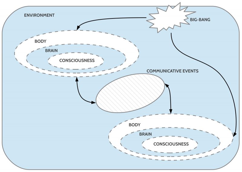
Within this self-replication, a semiotic process takes place—one that later, in the symbolic communication of highly complex organisms, particularly in Homo sapiens, became the foundation of an entirely new and highly efficient communication system between biological entities.
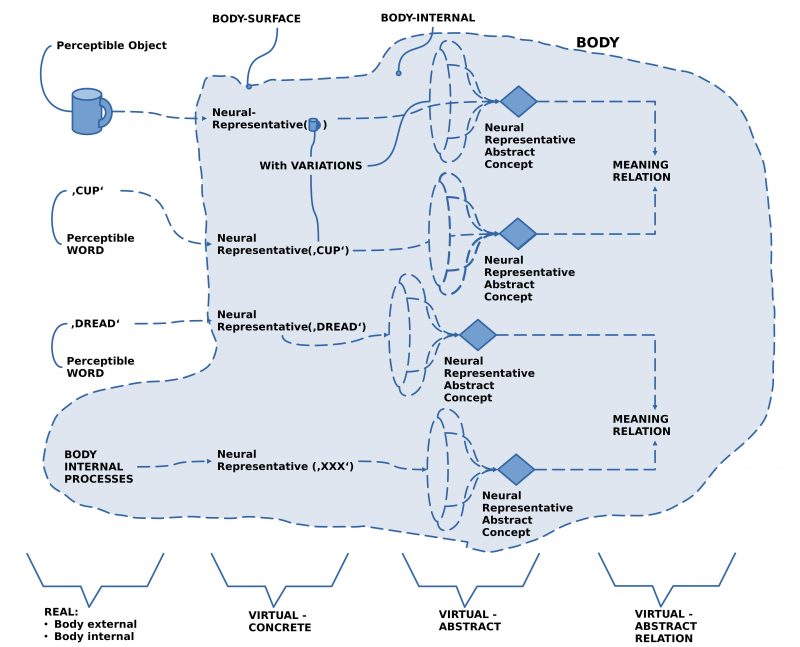
The Semiotic Structure of Life
The semiotic structure in the context of reproduction can be (simplified) as follows:
- One type of molecule (M1) interacts with another molecule (M2) as if the elements of M1 were control commands for M2.
- Through this interaction, M2 triggers chemical processes, which in turn lead to the construction of new molecules (M3).
- The elements of M1, which act like control commands, behave similarly to “signs” in semiotic theory.
- The molecules M3, produced by M2, can be understood semiotically as the “meaning” of M1—while M2 represents the “meaning relationship” between M1 and M3.
Not only the human brain operates with such semiotic structures, but every modern computer possesses them as well. This suggests that it may represent a universal structure.
Does Biological Matter Reveal Hidden Properties of Energy?
If we accept these considerations, then biological matter appears to differ from non-biological matter in the following aspects:
- Biological matter possesses the ability to arrange non-biological matter in such a way that functional relationships emerge between individual non-biological elements (atoms, molecules).
- These relationships can be interpreted as semiotic structures: Non-biological elements function “in context” (!) as “signs”, as “dynamic meaning relationships”, and as “meanings” themselves.
This raises an important question:
To what extent should the “additional properties” exhibited by biological matter be understood not only as “emergent properties” but also as manifestations of fundamental properties of energy itself?
Since energy e itself cannot be directly observed, only its effects can be studied. This leaves science with a choice:
- It can continue to adhere to the traditional perspective derived from Einstein’s 1905 formula e = mc²—but this means accepting that the most complex properties of the universe remain unexplained.
- Or, science can expand its perspective to include non-living matter in the form of biological systems, thereby integrating biological processes into the study of fundamental physics.
Biological systems cannot be explained without energy. However, their threefold structure—
- Matter as “objects,”
- Matter as a “meta-level,”
- Matter as an “actor”—
suggests that energy itself may possess far more internal properties than previously assumed.
Is this reluctance to reconsider energy’s role merely the result of a “false intellectual pride”? A refusal to admit that “in matter itself,” something confronts us that is far more than just “non-living matter”?
And yet, the observer—the knower—is exactly that: “matter in the form of biological systems” with properties that far exceed anything physics has been willing to account for so far.
And what about emotions?
- Throughout this discussion, emotions have barely been mentioned.
- What if energy is also responsible for this complex domain?
Maybe we all—philosophers, scientists, and beyond—need to go back to the start.
Maybe we need to learn to tell the story of life on this planet and the true meaning of being human in a completely new way.
After all, we have nothing to lose.
All our previous narratives are far from adequate.
And the potential future is, without a doubt, far more exciting, fascinating, and rich than anything that has been told so far…
APPENDIX
With the support of ChatGPT-4o, I tested a wide range of estimation functions (e.g., power function, inverted power function, exponential function, hyperbolic function, Gompertz function, logistic function, summed power function, each with different variations). As a result, the logistic (S-curve) function proved to be the one that best fit the real data values and allowed for a conservative estimate for the future, which appears reasonably plausible and could be slightly refined if necessary. However, given the many open parameters for the future, a conservative estimate seems to be the best approach: a certain direction can be recognized, but there remains room for unexpected events.
The following Python program was executed using the development environment Python 3.12.3 64-bit with Qt 5.15.13 and PyQt5 5.15.10 on Linux 6.8.0-52-generic (x86_64). (For Spyder, see: Spyder-IDE.org)
#!/usr/bin/env python3
# -*- coding: utf-8 -*-
"""
Created on Mon Feb 10 07:25:38 2025

@author: gerd (supported by chatGPT4o)
"""
import numpy as np
import pandas as pd
import matplotlib.pyplot as plt
from scipy.optimize import curve_fit

# Daten für die Tabelle
data = {
    "Phase": [
        "Molekulare Evolution zu Prokaryoten",
        "Prokaryoten zum Großen Sauerstoffereignis",
        "Sauerstoffereignis zu Eukaryoten",
        "Eukaryoten zu Vielzellern",
        "Vielzeller zu Homo",
        "Homo zu Homo sapiens",
        "Homo sapiens zu KI"
    ],
    "Dauer (Jahre)": [
        400e6,
        1e9,
        1e9,
        900e6,
        597.5e6,
        2.2e6,
        297900
    ]
}

# Gesamtzeit der Entwicklung des Lebens (ca. 3,9 Mrd. Jahre)
total_time = 3.9e9

# DataFrame erstellen
df = pd.DataFrame(data)

# Berechnung des prozentualen Anteils
df["% Anteil an Gesamtzeit"] = (df["Dauer (Jahre)"] / total_time) * 100

# Berechnung der kumulativen Zeit
df["Kumulative Zeit (Mrd. Jahre)"] = (df["Dauer (Jahre)"].cumsum()) / 1e9

# Extrahieren der relevanten kumulativen Zeitintervalle (Differenzen der biologischen Phasen)
relevant_intervals = df["Kumulative Zeit (Mrd. Jahre)"].iloc[1:6].diff().dropna().values

# Definieren der Zeitindices für die relevanten Intervalle
interval_steps = np.arange(len(relevant_intervals))


# Sicherstellen, dass x_cumulative_fit korrekt definiert ist
x_cumulative_fit = np.arange(1, 6)  # Index für biologische Phasen 1 bis 5
y_cumulative_fit = df["Kumulative Zeit (Mrd. Jahre)"].iloc[1:6].values  # Die zugehörigen Zeiten

# Logistische Funktion (Sigmoid-Funktion) definieren
def logistic_fit(x, L, x0, k):
    return L / (1 + np.exp(-k * (x - x0)))  # Standardisierte S-Kurve

# Curve Fitting für die kumulierte Zeitreihe mit der logistischen Funktion
params_logistic, _ = curve_fit(
    logistic_fit,
    x_cumulative_fit,
    y_cumulative_fit,
    p0=[max(y_cumulative_fit), np.median(x_cumulative_fit), 1],  # Startwerte
    maxfev=2000  # Mehr Iterationen für stabilere Konvergenz
)

# Prognose des nächsten kumulierten Zeitpunkts mit der logistischen Funktion
predicted_cumulative_logistic = logistic_fit(len(x_cumulative_fit) + 1, *params_logistic)

# Fit-Kurve für die Visualisierung der logistischen Anpassung
x_fit_time_logistic = np.linspace(1, len(x_cumulative_fit) + 1, 100)
y_fit_time_logistic = logistic_fit(x_fit_time_logistic, *params_logistic)

# Visualisierung der logistischen Anpassung an die kumulierte Zeitreihe
plt.figure(figsize=(10, 6))
plt.scatter(x_cumulative_fit, y_cumulative_fit, color='blue', label="Real Data Points")
plt.plot(x_fit_time_logistic, y_fit_time_logistic, 'r-', label="Logistic Fit (S-Curve)")
plt.axvline(len(x_cumulative_fit) + 1, color='r', linestyle='--', label="Next Forecast Point")
plt.scatter(len(x_cumulative_fit) + 1, predicted_cumulative_logistic, color='red', label=f"Forecast: {predicted_cumulative_logistic:.3f} Bn Years")

# Titel und Achsenbeschriftungen
plt.title("Logistic (S-Curve) Fit on Cumulative Evolutionary Time")
plt.xlabel("Evolutionary Phase Index")
plt.ylabel("Cumulative Time (Billion Years)")
plt.legend()
plt.grid(True)
plt.show()

# Neues t_next basierend auf der logistischen Anpassung
predicted_cumulative_logistic

Out[109]: 4.04682980616636 (Prognosewert)