QUANTUM THEORY (QT). BASIC PROPERTIES

eJournal: uffmm.org, ISSN 2567-6458, 31.Dec. 2018
Email: info@uffmm.org
Author: Gerd Doeben-Henisch
Email: gerd@doeben-henisch.de

CONTEXT

This is a continuation from the post BACKGROUND INFORMATION 27.Dec.2018: The AAI-paradigm and Quantum Logic. The Limits of Classic Probability. The general topic here is the analysis of properties of human behavior, actually narrowed down to the statistical properties. From the different possible theories applicable to statistical properties of behavior one is called CPT (classical probability theory), see the before mentioned post, and the other QLPT (quantum logic probability theory), which will be discussed now.

SUMMARY

First description of what Quantum Theory QT) is which is implying  quantum logic.

QT AND REALITY

To approach the topic of QLTP we will start from a philosophy of science point of view beginning with the general question of the relation between ‘quantum theory (QT)’ and ‘reality’ (here we follow Griffiths (2003) in his final reflections about QT in chapter 27 of his book).

  1. Griffiths makes the clear distinction between QT as a theory (T) and something we call real world (W) or physical reality which is clearly distinct from the theory.
  2. A theory is realized as a set of symbolic expressions which are assumed to have a relation to the presupposed real world. The symbolic matter as such is not the theory but those structures in the mind of the scientists which are comprehended. In our mind – something ‘inside’ our body; usually located in the brain – we can in an abstract way distinguish elements and relations between these elements. Furthermore we can think about these elements and relations on a meta level and define concepts like ‘is coherent’, ‘is logical’, ‘is beautiful’.
  3. Besides the definitions ‘inside the mind’ about ‘elements already in the mind’ (like ‘consistency’ …) there exists the question of the confirmation of theoretical constructs compared to the real world as it is. As we know there exist one primary mode of relationship and some secondary mode to interact with the presupposed ‘real world’:
    1. The primary mode is the sensory perception, which generates typical internal events in the brain, and
    2. the secondary mode is a sensory perception in cooperation with defined measurement procedures. Thus the measurement results are as such not different to other sensory perceptions but the measurement results are generated by a certain procedure which can be repeated from everybody who wants to look to the measurement results again, and this procedure is using a before agreed measurement standard object to give a point of reference for everybody.
  4. The possible confirmation of theoretical constructs t of some theory T by measurements requires the availability of appropriate measurements communicated to the mind through the sensory perception and some mapping between the sensory data and the theoretical constructs. Usually the sensory data are by themselves not raw data but are symbolic expressions ‘representing the data in a symbolic format’. Thus the mapping in the mind has to connect the perceptions of the symbolic measurement with parts of the theory.
  5. Because it is assumed that the theory is also encoded in symbolic expressions for communication one has to assume that one has to distinguish between the symbolic representation of the theory and their domain of application consisting of elements and relations generated in the mind. In modern formal theories the relationship between measurement expressions and theoretical expressions is defined in an appropriate logic describing possible inferences which deliver within a logical proof either a formal confirmation or not.
  6. As Griffiths remarks the different confirmations of individual measurements do not guarantee the truth of the theory saying that the assumed theory is an adequate description of the presupposed real world. This results from the fact that every experimental confirmation can only give very partial confirmations compared to the nearly infinite space of possible statements which are entailed by a modern theory. Therefore it is finally a question of faith whether some proposed empirical theory is gaining acceptance and is used ‘as if it is true’. This means the theory can be refuted at any time point in the future.
  7. For the QT Griffiths claims that nearly everybody today accepts QT as the best available theory about the real world.(cf. p.361)
  8. Within QT the dynamical laws are inherently stochastic/ probabilistic, this means that the future behavior of a quantum system cannot be predicted with certainty. (cf. Griffiths (2003):p.362)
  9. The reason for this unpredictability is that the elementary objects of the QT, the ‘quantum particles‘, have no precise position or momentum. A precise description of these particles is limited by the Heisenberg uncertainty principle. (cf. Griffiths (2003):p.361)
  10. This inherent property of QT of having objects with no clear position and momentum allows the further fact that there can be different formalism logically incompatible with each other but nevertheless describing a certain aspect of the QT domain in a ‘sound’ manner. (cf. Griffiths (2003):pp.262-265)
  11. While the interaction of a quantum system can be described, the ‘decoherence‘ of a macroscopic quantum superposition (MQS) state can directly not be measured. To enable a theoretic description for this properties requires concepts and a language which deviates from everyday experiences, concepts, and languages. (cf. Griffiths (2003):pp.265-268)
  12. Summing up one gets the following list of important properties looking to an presupposed ‘independent real world’ (cf. Griffiths (2003):p.268f):
    1. Physical objects never possess a completely precise position or momentum.
    2. The fundamental dynamical laws of physics are stochastic and not deterministic.
    3. There is not a unique exhaustive description of a physical system or a physical process.
    4. Quantum measurements can be understood as revealing properties of a measured system before the measurement took place, in a manner which was taken for granted in classical physics.
    5. Quantum mechanics is a local theory in the sense that the world can be understood without supposing that there are mysterious influences which propagate over long distances more rapidly than the speed of light.
    6. Quantum mechanics is consistent with the notion of an independent reality, a real world whose properties and fundamental laws do not depend upon what human beings happen to believe, desire, or think.

Taking these assumptions for granted one has to analyze now what this implies for the description and computation of the behavior of states of properties generated by biological systems.

See a continuation here.

REFERENCES

  • R.B. Griffiths. Consistent Quantum Theory. Cambridge University Press, New York, 2003


SIMPLE PROGRAMMING ENVIRONMENT WITH PYTHON-SPYDER

eJournal: uffmm.org, ISSN 2567-6458, 30.Dec 2018; extension 10.April 2019
Email: info@uffmm.org
Author: Gerd Doeben-Henisch
Email: gerd@doeben-henisch.de

CONTEXT

This post is part of the online book project for the AAI-paradigm. As mentioned in the text of the book the AAI paradigm will need for its practical usage appropriate software. Some preliminary (experimentally) programming is already underway. The programming language used for this programming is python. Here some bits of information how one can install a simple python environment to share these activities.

WINPYTHON OR ANACONDA WITH SPYDER
(Windows as well as Linux (ubuntu))

To work with the python programming language — here python 3 —  one needs some tools interacting with each other. For this different integrated development packages have been prepared.  In this uffmm-software project I am using the spyder development environment either as part of the winpython distribution or as part of the anaconda distribution.

WINPYTHON DISTRIBUTION

The winpython package can be found here. See also the picture below.

Website of winpython distribution

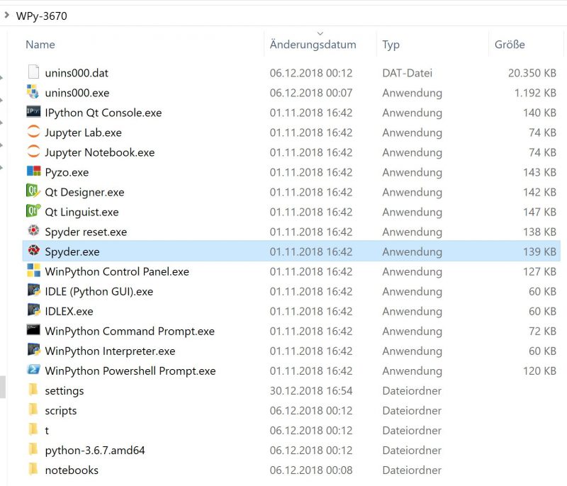
If one has downloaded the winpython distribution in some local folder then you will see the following files and folders (see picture below):

winpython distribution folder after installation

SPYDER INTEGRATED ENVIRONMENT

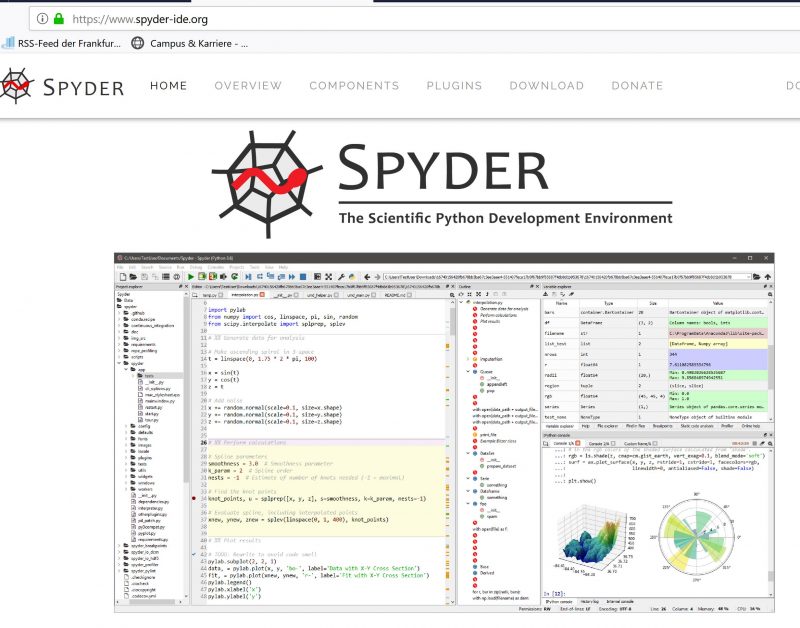
To use the integrated spyder environment one can also look to the spyder website directly (see picture below).

spyder working environment for python - website
spyder working environment for python – website

The spyder team recomments to download the spyder software as part of the bigger anaconda distribution with lots of additional options (see picture below).

spyder working environment embedded in the anaconda distribution

Downloading the anaconda distribution needs much more time then the winpython distribution. But one gets a lot of stuff and the software is fairly good integrated into the windows 10 operating system. I personally recomment for the beginners not to beginn with the complex anaconda environment but to stay with the spyder integrated environment only. This can be done by activating with the windows-button the list of apps, looking to the anaconda icon, and there one can find the spyder icon (an idealized spyder web). One can click with the right mouse button on this icon and then select to ‘add to the task bar’. After this operation you can observe the spyder icon as attached to the task bar like in the picture below.

part of the task bar in windows with icons for spyder and a python environment
Part of the task bar in windows with icons for spyder (right border)  and a python environment (left from spyder)

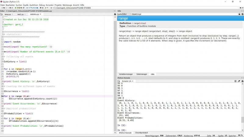
If one activates the spyder icon a window opens showing some standard configuration of the integrated spyder development environment (see picture below).

spyder working environment with editor, console, and additional object informations

The most important sub-windows are the window left from the editor and the window right-below from the console.  One can use the console to make small experiments with python commands and the editor to write larger source code.  In the header bar are many helpful icons for editing, running of programs, testing, and more.

LINUX (UBUNTU)

If one is working with linux (what I am usually are doing; I use the distribution ubuntu 18.04.1 LTS) then python is part of the system in version 2 as well in version 3 and spyder can be used too.

WINPYTHON CONSOLE

Besides the integrated development editor (IDE) spyder you can find even more programming tools. One very helpful tool is the WinPython Console (see icon within the red circle). You can attach this icon on your task bar too and then you can start the Winpython Console by clicking on it.

Figure 1: Directory path after starting the WinPython Console

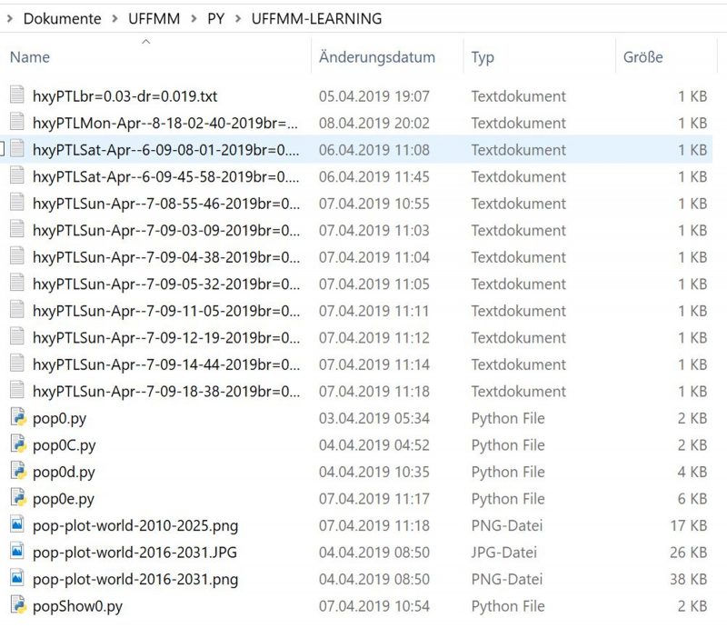
To apply this console to some python programm you have to navigate to that folder where you have the python program to be executed. If You do not know already the whole path then you have two options: (i) move the path upwards by using the command ‘cd ..’ (change directory one level upwards) or (ii) move the path downwards by using the command ‘cd DIR-NAME‘. If you are in a new folder you can use the command ‘dir‘ to list all the files and folders in the actual directory. Doing this You can reach the following folder with some python program files:

Figure 2: Folder with some python programs

There is one example file pop0e.py which we can start (the whole program will be described later in detail).

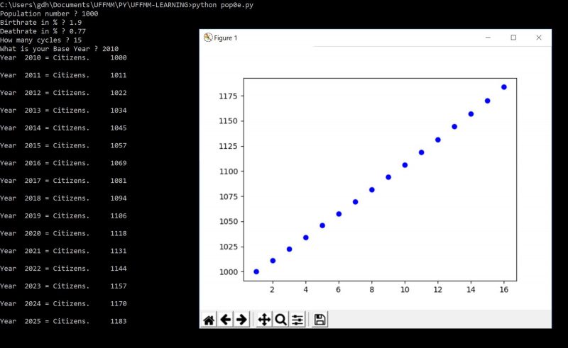
Figure 3: Shows an example run with the program pop0e.py, some print outs as well as a diagram.

For this last example with the Winpython Console the program can be edited by nearly any kind of a text editor. After the file has been saved with a .py ending one can use the console to start the program. In the last example (cf. figure 3) the important input was: ‘python pop0e.py‘ this states that the python interpreter shall take the program text of the file ‘pop0e.py’ and execute the program.

LEARNING ENVIRONMENT

For an overview of all posts in this block about programming with python 3 see HERE.

BACKGROUND INFORMATION 27.Dec.2018: The AAI-paradigm and Quantum Logic. The Limits of Classic Probability

eJournal: uffmm.org, ISSN 2567-6458
Email: info@uffmm.org
Author: Gerd Doeben-Henisch
Email: gerd@doeben-henisch.de

Last Corrections: 30.Dec.2018

CONTEXT

This is a continuation from the post about QL Basics Concepts Part 1. The general topic here is the analysis of properties of human behavior, actually narrowed down to the statistical properties. From the different possible theories applicable to statistical properties of behavior here the one called CPT (classical probability theory) is selected for a short examination.

SUMMARY

An analysis of the classical probability theory shows that the empirical application of this theory is limited to static sets of events and probabilities. In the case of biological systems which are adaptive with regard to structure and cognition this does not work. This yields the question whether a quantum probability theory approach does work or not.

THE CPT IDEA

  1. Before we are looking  to the case of quantum probability theory (QLPT) let us examine the case of a classical probability theory (CPT) a little bit more.
  2. Generally one has to distinguish the symbolic formal representation of a theory T and some domain of application D distinct from the symbolic representation.
  3. In principle the domain of application D can be nearly anything, very often again another symbolic representation. But in the case of empirical applications we assume usually some subset of ’empirical events’ E of the ’empirical (real) world’ W.
  4. For the following let us assume (for a while) that this is the case, that D is a subset of the empirical world W.
  5. Talking about ‘events in an empirical real world’ presupposes that there there exists a ‘procedure of measurement‘ using a ‘previously defined standard object‘ and a ‘symbolic representation of the measurement results‘.
  6. Furthermore one has to assume a community of ‘observers‘ which have minimal capabilities to ‘observe’, which implies ‘distinctions between different results’, some ‘ordering of successions (before – after)’, to ‘attach symbols according to some rules’ to measurement results, to ‘translate measurement results’ into more abstract concepts and relations.
  7. Thus to speak about empirical results assumes a set of symbolic representations of those events as a finite set of symbolic representations which represent a ‘state in the real world’ which can have a ‘predecessor state before’ and – possibly — a ‘successor state after’ the ‘actual’ state. The ‘quality’ of these measurement representations depends from the quality of the measurement procedure as well as from the quality of the cognitive capabilities of the participating observers.
  8. In the classical probability theory T_cpt as described by Kolmogorov (1932) it is assumed that there is a set E of ‘elementary events’. The set E is assumed to be ‘complete’ with regard to all possible events. The probability P is coming into play with a mapping from E into the set of positive real numbers R+ written as P: E —> R+ or P(E) = 1 with the assumption that all the individual elements e_i of E have an individual probability P(e_i) which obey the rule P(e_1) + P(e_2) + … + P(e_n) = 1.
  9. In the formal theory T_cpt it is not explained ‘how’ the probabilities are realized in the concrete case. In the ‘real world’ we have to identify some ‘generators of events’ G, otherwise we do not know whether an event e belongs to a ‘set of probability events’.
  10. Kolmogorov (1932) speaks about a necessary generator as a ‘set of conditions’ which ‘allows of any number of repetitions’, and ‘a set of events can take place as a result of the establishment of the condition’. (cf. p.3) And he mentions explicitly the case that different variants of the a priori assumed possible events can take place as a set A. And then he speaks of this set A also of an event which has taken place! (cf. p.4)
  11. If one looks to the case of the ‘set A’ then one has to clarify that this ‘set A’ is not an ordinary set of set theory, because in a set every member occurs only once. Instead ‘A’ represents a ‘sequence of events out of the basic set E’. A sequence is in set theory an ‘ordered set’, where some set (e.g. E) is mapped into an initial segment  of the natural numbers Nat and in this case  the set A contains ‘pairs from E x Nat|\n’  with a restriction of the set Nat to some n. The ‘range’ of the set A has then ‘distinguished elements’ whereby the ‘domain’ can have ‘same elements’. Kolmogorov addresses this problem with the remark, that the set A can be ‘defined in any way’. (cf. p.4) Thus to assume the set A as a set of pairs from the Cartesian product E x Nat|\n with the natural numbers taken from the initial segment of the natural numbers is compatible with the remark of Kolmogorov and the empirical situation.
  12. For a possible observer it follows that he must be able to distinguish different states <s1, s2, …, sm> following each other in the real world, and in every state there is an event e_i from the set of a priori possible events E. The observer can ‘count’ the occurrences of a certain event e_i and thus will get after n repetitions for every event e_i a number of occurrences m_i with m_i/n giving the measured empirical probability of the event e_i.
  13. Example 1: Tossing a coin with ‘head (H)’ or ‘tail (T)’ we have theoretically the probabilities ‘1/2’ for each event. A possible outcome could be (with ‘H’ := 0, ‘T’ := 1): <((0,1), (0,2), (0,3), (1,4), (0,5)> . Thus we have m_H = 4, m_T = 1, giving us m_H/n = 4/5 and m_T/n = 1/5. The sum yields m_H/n + m_T/n = 1, but as one can see the individual empirical probabilities are not in accordance with the theory requiring 1/2 for each. Kolmogorov remarks in his text  that if the number of repetitions n is large enough then will the values of the empirically measured probability approach the theoretically defined values. In a simple experiment with a random number generator simulating the tossing of the coin I got the numbers m_Head = 4978, m_Tail = 5022, which gives the empirical probabilities m_Head/1000 = 0.4977 and m_Teil/ 1000 = 0.5021.
  14. This example demonstrates while the theoretical term ‘probability’ is a simple number, the empirical counterpart of the theoretical term is either a simple occurrence of a certain event without any meaning as such or an empirically observed sequence of events which can reveal by counting and division a property which can be used as empirical probability of this event generated by a ‘set of conditions’ which allow the observed number of repetitions. Thus we have (i) a ‘generator‘ enabling the events out of E, we have (ii) a ‘measurement‘ giving us a measurement result as part of an observation, (iii) the symbolic encoding of the measurement result, (iv) the ‘counting‘ of the symbolic encoding as ‘occurrence‘ and (v) the counting of the overall repetitions, and (vi) a ‘mathematical division operation‘ to get the empirical probability.
  15. Example 1 demonstrates the case of having one generator (‘tossing a coin’). We know from other examples where people using two or more coins ‘at the same time’! In this case the set of a priori possible events E is occurring ‘n-times in parallel’: E x … x E = E^n. While for every coin only one of the many possible basic events can occur in one state, there can be n-many such events in parallel, giving an assembly of n-many events each out of E. If we keeping the values of E = {‘H’, ‘T’} then we have four different basic configurations each with probability 1/4. If we define more ‘abstract’ events like ‘both the same’ (like ‘0,0’, ‘1,1’) or ‘both different’ (like ‘0,1’. ‘1,0’), then we have new types of complex events with different probabilities, each 1/2. Thus the case of n-many generators in parallel allows new types of complex events.
  16. Following this line of thinking one could consider cases like (E^n)^n or even with repeated applications of the Cartesian product operation. Thus, in the case of (E^n)^n, one can think of different gamblers each having n-many dices in a cup and tossing these n-many dices simultaneously.
  17. Thus we have something like the following structure for an empirical theory of classical probability: CPT(T) iff T=<G,E,X,n,S,P*>, with ‘G’ as the set of generators producing out of E events according to the layout of the set X in a static (deterministic) manner. Here the  set E is the set of basic events. The set X is a ‘typified set’ constructed out of the set E with t-many applications of the Cartesian operation starting with E, then E^n1, then (E^n1)^n2, …. . ‘n’ denotes the number of repetitions, which determines the length of a sequence ‘S’. ‘P*’ represents the ’empirical probability’ which approaches the theoretical probability P while n is becoming ‘big’. P* is realized as a tuple of tuples according to the layout of the set X  where each element in the range of a tuple  represents the ‘number of occurrences’ of a certain event out of X.
  18. Example: If there is a set E = {0,1} with the layout X=(E^2)^2 then we have two groups with two generators each: <<G1, G2>,<G3,G4>>. Every generator G_i produces events out of E. In one state i this could look like  <<0, 0>,<1,0>>. As part of a sequence S this would look like S = <….,(<<0, 0>,<1,0>>,i), … > telling that in the i-th state of S there is an occurrence of events like shown. The empirical probability function P* has a corresponding layout P* = <<m1, m2>,<m3,m4>> with the m_j as ‘counter’ which are counting the occurrences of the different types of events as m_j =<c_e1, …, c_er>. In the example there are two different types of events occurring {0,1} which requires two counters c_0 and c_1, thus we would have m_j =<c_0, c_1>, which would induce for this example the global counter structure:  P* = <<<c_0, c_1>, <c_0, c_1>>,<<c_0,  c_1>,<c_0, c_1>>>. If the generators are all the same then the set of basic events E is the same and in theory   the theoretical probability function P: E —> R+ would induce the same global values for all generators. But in the empirical case, if the theoretical probability function P is not known, then one has to count and below the ‘magic big n’ the values of the counter of the empirical probability function can be different.
  19. This format of the empirical classical  probability theory CPT can handle the case of ‘different generators‘ which produce events out of the same basic set E but with different probabilities, which can be counted by the empirical probability function P*. A prominent case of different probabilities with the same set of events is the case of manipulations of generators (a coin, a dice, a roulette wheel, …) to deceive other people.
  20. In the examples mentioned so far the probabilities of the basic events as well as the complex events can be different in different generators, but are nevertheless  ‘static’, not changing. Looking to generators like ‘tossing a coin’, ‘tossing a dice’ this seams to be sound. But what if we look to other types of generators like ‘biological systems’ which have to ‘decide’ which possible options of acting they ‘choose’? If the set of possible actions A is static, then the probability of selecting one action a out of A will usually depend from some ‘inner states’ IS of the biological system. These inner states IS need at least the following two components:(i) an internal ‘representation of the possible actions’ IS_A as well (ii) a finite set of ‘preferences’ IS_Pref. Depending from the preferences the biological system will select an action IS_a out of IS_A and then it can generate an action a out of A.
  21. If biological systems as generators have a ‘static’ (‘deterministic’) set of preferences IS_Pref, then they will act like fixed generators for ‘tossing a coin’, ‘tossing a dice’. In this case nothing will change.  But, as we know from the empirical world, biological systems are in general ‘adaptive’ systems which enables two kinds of adaptation: (i) ‘structural‘ adaptation like in biological evolution and (ii) ‘cognitive‘ adaptation as with higher organisms having a neural system with a brain. In these systems (example: homo sapiens) the set of preferences IS_Pref can change in time as well as the internal ‘representation of the possible actions’ IS_A. These changes cause a shift in the probabilities of the events manifested in the realized actions!
  22. If we allow possible changes in the terms ‘G’ and ‘E’ to ‘G+’ and ‘E+’ then we have no longer a ‘classical’ probability theory CPT. This new type of probability theory we can call ‘non-classic’ probability theory NCPT. A short notation could be: NCPT(T) iff T=<G+,E+,X,n,S,P*> where ‘G+’ represents an adaptive biological system with changing representations for possible Actions A* as well as changing preferences IS_Pref+. The interesting question is, whether a quantum logic approach QLPT is a possible realization of such a non-classical probability theory. While it is known that the QLPT works for physical matters, it is an open question whether it works for biological systems too.
  23. REMARK: switching from static generators to adaptive generators induces the need for the inclusion of the environment of the adaptive generators. ‘Adaptation’ is generally a capacity to deal better with non-static environments.

See continuation here.

BACKGROUND INFORMATION 27.Dec.2018: The AAI-paradigm and Quantum Logic. Basic Concepts. Part 1

eJournal: uffmm.org, ISSN 2567-6458
Email: info@uffmm.org
Author: Gerd Doeben-Henisch
Email: gerd@doeben-henisch.de

Some corrections: 28.Dec.2018

As mentioned in a preceding post the AAI paradigm has to be reconsidered in the light of the quantum logic (QL) paradigm. Here some first concepts which have to be considered (see for the following text chapter two of the book: Jerome R. Busemeyer and Peter D. Bruza, Quantum Models of Cognition and Decision, Cambridge University Press, Cambridge (UK), 2012).

The paradigms of ‘quantum logic’ as well as ‘quantum probability theory’ arose in the field of physics, but as it became clear later these formalisms can be applied to other domains than physics too.

The basic application domain is a appears as a paradigm – real or virtual – in which one can distinguish ‘events‘ which can ‘occur‘ along a time-line as part of a bigger state. The ‘frequency‘ of the occurrences of the different events can be ‘counted’ as a function of the presupposed time-line. The frequency can be represented by a ‘number‘. The frequency can be a ‘total frequency’ for the ‘whole time-line’ or a ‘relative frequency’ with regard to some part of a ‘partition of the time-line’. Having relative frequencies these can possibly ‘change‘ from part to part.

The basic application domain can be mapped into a formalism which ‘explains’ the ‘probability’ of the occurrences of the events in the application domain. Such a formalism is an ‘abstraction’ or an ‘idealization‘ of a certain type of an application domain.

The two main types of formalisms dealt with in the mentioned book of Busemeyer and Bruza (2012) are called ‘classical probability theory’ and ‘quantum probability theory’.

The classical theory of probability (CTP)has been formalized as a theory in the book by A.N. Kolmogorov, Foundations of the Theory of Probability. Chelsea Publ. Company, New York, 2nd edition, 1956 (originally published in German 1933). The quantum logic version of the theory of probability (QLTP) has been formalized as a theory in the book John von Neumann, Mathematische Grundlagen der Quantenmechanik, published by Julius Springer, Berlin, 1932 (a later English version has been published 1956).

In the CTP the possible elementary events are members of a set E which is mapped into the set of positive real numbers R+. The probability of an event A is written as P(A)=r (with r in R*). The probability of the whole set E is assumed as P(E) = 1. The relationship between the formal theory CTP and the application domain is given by a mapping of the abstract concept of probability P(A) to the relation between the number of repetitions of some mechanism of event-generation n and the number of occurrences m of a certain event A written as n/m. If the number of repetitions is ‘big enough’, then – according to Kolmogorov — the relation ‘n/m’ will differ only slightly from the theoretical probability P(A) (cf. Kolmogorov (1956):p.4)

The expression ‘mechanism of event-generation‘ is very specific; in general we have a sequence of states along a time-line and some specific event A can occur in one of these states or not. If event A occurs then the number m of occurrences m is incremented while the number of repetitions n corresponds to the number of time points which are associated with a state of a possible occurrence counted since a time point declared as a ‘starting point‘ for the observation. Because time points in an application domain are related to machines called ‘clocks‘ the ‘duration‘ of a state is related to the ‘partition’ of a time unit like ‘second [s]’ realized by the used clock. Thus depending from the used clock can the number of repetitions become very large. Compared to the human perception can this clock-based number of repetitions be ‘misleading’ because a human observer has seen perhaps only two occurrences of the event A while the clock measured some number n* far beyond two. This short remark reveals that the relationship between an abstract term of ‘probability’ and an application domain is far from trivial. Basically it is completely unclear what theoretical probability means in the empirical world without an elaborated description of the relationship between the formal theory and the sequences of events in the real world.

See next.


BACKGROUND INFORMATION 24.Dec.2018: The AAI-pParadigm and Quantum Logic

eJournal: uffmm.org, ISSN 2567-6458
Email: info@uffmm.org
Author: Gerd Doeben-Henisch
Email: gerd@doeben-henisch.de

Extending the main page another important idea has to be noticed: quantum logic, originally created in the realm of modern physics, has brought forward a formalism  dealing with superposition states (states of substantial uncertainty for the observer). This formalism has meanwhile entered other disciplines, especially disciplines dealing with cognition and decision processes (see as an excellent example the book: Jerome R. Busemeyer and Peter D. Bruza, Quantum Models of Cognition and Decision, Cambridge University Press, Cambridge (UK), 2012).

As it turns out there is a bad and a good message for the AAI paradigm: the ‘bad’ message is, that the AAI formalism so far is written in a non-quantum logic style. Thus it seems as if the AAI paradigm is stuck with the classical pre-quantum view of the world. The ‘good’ message is, that this ‘pre-quantum’ style is only at the ‘surface’ of the AAI paradigm. If one considers the ‘actor models’ – which are a substantial component of the AAI paradigm – as ‘truly quantum-like systems‘ (what they are in the ‘normal case’), then one can think of the ‘actors’ as systems having three components at least: (i) a biological basis (or some equivalent matter) consisting of highly entangled quantum systems, which are organized as ‘biological bodies‘ with a brain; (ii) a ‘consciousness‘ interacting with (iii) an ‘unconsciousness‘. The consciousness is heavily depending from the behavior of the unconsciousness in a way which resembles a superposition state! By ‘learning‘ the system can store some ‘procedures’ for later activation in the unconsciousness, but the stored procedures (a) can not override the superposition state completely and (b) the stored procedures are not immune against changes in time. Thus from the point of ‘decisions’ and of ‘thinking’ an actor is always an inherently in-deterministic system which can better be described with a quantum-logic similar formalism than with a non-quantum-logic formalism.

In general one should abandon the term ‘quantum’ from the formalism because the domain of reference are not some physical ‘quanta’ below the atoms but complete learning systems with a stochastic unconsciousness as basis for learning.

To implement these quantum logic perspective into the AAI paradigm does not change the paradigm as a whole but primarily the descriptions of the participating actors.

As a consequence of this change the simulation process has to be seen in a new way:  because every participating actor is a truly indeterministic  system, the whole state at some time point t is a superposition state. Therefore  every concrete simulation is a ‘selection’ of ‘one path out of many possible ones’. Thus a concrete  simulation  can only show one fragment of an unknown bigger space of possible other runs. And their is another point: because all actors are ‘learning’ actors in the unrestricted sense (known artificial intelligence systems today are strongly restricted learners!) the actors in the process are ‘changing’. Thus an actor at time point t+x is not the same as the actor with the same ‘name’ at an earlier time point t! To draw conclusions about possible ‘repetitions in the future’ is therefore dangerous. The future in a quantum-like world will never repeat the past.

See next.

BACKGROUND INFORMATION 19.Dec.2018: The e-Politics Project

eJournal: uffmm.org, ISSN 2567-6458
Email: info@uffmm.org
Author: Gerd Doeben-Henisch
Email: gerd@doeben-henisch.de

If You are wondering why no new updates appear on the main page the reason why is, that some heavy work is going on in the background using the AAI paradigm published here so far within a German course  called Mensch-Maschine Interaktion (MMI) in the Frankfurt University of Applied Sciences (FRA-UAS) as well in a growing interdisciplinary project where the AAI paradigm is applied to the topic of ‘communal planning using e-gaming’. Because both activities are in German there is time lacking to continue writing in English :-). In the context of the ‘communal planning with e-gaming’  project  we are planning to do some more field-experiments in the upcoming months with ‘normal citizens’ using these methods as a ‘bottom-up strategy’ for getting shared models of their cities which can be simulated. It is highly probable that a small booklet in German will appear to support these experiments before this English version will be expanded.

During  the time since Nov-4, 2018  the theory of the AAI paradigm could be improved in many points (documented in the German texts) and meanwhile I have started to program a first version of a software (in python) by myself. Doing this the experience is always the same: You think You ‘know’ the subject matter’ because You have written some texts with formulas, but if You are starting programming, You are challenged in a much more concrete way. Without theory the programming wouldn’t know what to do,  but without programming you will never understand in a sufficient concrete way what You are thinking