Category Archives: actor model (AM)

HMI ANALYSIS, Part 4: Tool based Actor Story Development with Testing and Gaming

Integrating Engineering and the Human Factor (info@uffmm.org)
eJournal uffmm.org ISSN 2567-6458, March 3-4, 2021,
Author: Gerd Doeben-Henisch
Email: gerd@doeben-henisch.de

Last change: March 4, 2021, 07:49h (Minor corrections; relating to the UN SDGs)

HISTORY

As described in the uffmm eJournal  the wider context of this software project is an integrated  engineering theory called Distributed Actor-Actor Interaction [DAAI] further extended to the Collective Man-Machine Intelligence [CM:MI] paradigm.  This document is part of the Case Studies section.

HMI ANALYSIS, Part 4: Tool based Actor Story Development with Testing and Gaming

Context

This text is preceded by the following texts:

INFO GRAPH

Overview about different scenarios which will be possible for the development, simulation, testing and gaming of actor stories using the oksimo software tool

Introduction

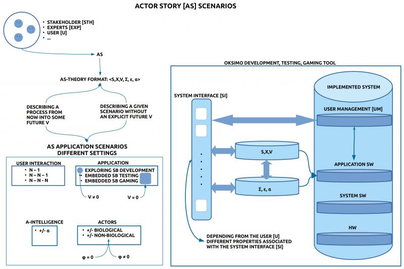
In the preceding post it has been explained, how one can format an actor story [AS] as a theory in the  format  of  an Evaluated Theory Tε with Algorithmic Intelligence:   Tε,α=<M,∑,ε,α>.

In the following text it will be explained which kinds of different scenarios will be possible to elaborate, to simulate, to test, and to enable gaming with  an actor story theory by using the oksimo software tool.

UNIVERSAL TEAM

The classical distinctions between certain types of managers, special experts and the rest of the world is given up here in favor of a stronger generalization: everybody is a potential expert with regard to a future, which nobody knows. This is emphasized by the fact, that everybody can use its usual mother tongue, a normal language, every language. Nothing more is needed.

BASIC MODELS (S, X)

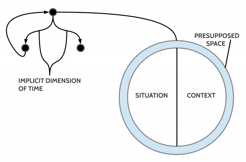
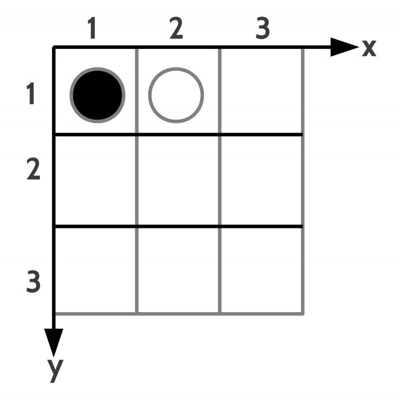
As minimal elements for all possible applications it is assumed here that the experts define at least a given situation (state) [S] and a set of change rules [X].

The given state S is  either (i)  taken as it is or (ii)  as a state which  should be improved. In both cases the initial state S is called the start state [S0].

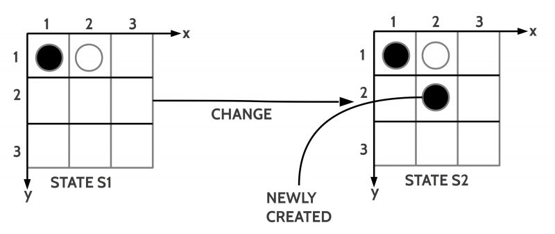
The change rules X describe possible changes which transform a given state S into a changed successor state S’.

A pair of S and X as (S,X) is called a basic model M(S,X). One can define as many models as one wants.

A DIRECTION BY A VISION V

A vision [V] can describe a possible state SV  in an assumed future. If such a state SV is given, then this state becomes a goal state SGoal In this case  we assume V ≠ 0. If no explicit goal is given, then we assume V = 0.

DEVELOPMENT BY GOALS

If a vision is given (V ≠ 0), then the vision can be used to induce a direction which can/ shall be approached by creating a set X, which enables the generation of a sequence of states with the start state S0 as first state followed by successor state Si until the goal state SGoal has been reached or at least it holds that the goal state is a subset of the reached state: SGoalSn.

It is possible to use many basic models M(S,X) in parallel and for each model Mi one can define a different goal Vi (the typical situation in a pluralistic society).

Thus there can be many basic theories T(M,V) in parallel.

STEADY STATES (V = 0)

If no explicit visions are defined (V = 0) then every direction of change is allowed. A basic steady state theory T(M,V) with V = 0 can   be written as T(M,0). Whether such a case can be of interest is not clear at the moment.

BASIC INTERACTION PATTERNS

The following interaction modes are assumed as typical cases:

  1. N-1: Within an online session an interactive webpage with the oksimo software is active and the whole group can interact with the oksimo software tool.
  2. N-N-1: N-many participants can individually login into the interactive oksimo website and being logged in they can collaborate within the oksimo software with one project.
  3. N-N-N: N-many participants can individually login into the interactive oksimo website and there everybody can run its own process or can collaborate in various ways.

The default case is case (1). The exact dates for the availability of modes (2) – (3) depends from how fast the roadmap can be realized.

BASIC APPLICATIONS
  1. Exploring Simulation-Based Development [ESBD] (V ≠ 0): If the main goal is to find a path from a given state today S (Now) to an envisioned state V in the future then one has  to collect appropriate change rules X to approach the final goal state SGoal better and better. Activating the simulator ∑ during search and construction phase at will can be of great help, especially if the documents (S, X, V) are becoming more and more complex.
  2. Embedded Simulation-Based  Testing [ESBT] (V ≠ 0): If a basic  actor story theory T(M,) is given with a given goal (V ≠ 0) then it is of great help if the simulation is done in interactive mode where the simulator is not applying the change rules by itself but by asking different logged in users which rule they want to apply and how. These tests show not only which kinds of errors will occur but they can also show during n-many repetitions to which degree an user  can learn to behave task-conform. If the tests will not show the expected outcomes then this can point  to possible deficiencies of the software as well to specialties of the user.
  3. Embedded Simulation-Based Gaming [ESBTG] (V ≠ 0):  The case of gaming is partially  different to the case of testing.  Although it is assumed here too that at least one vision (goal) is given, it is additionally assumed that  there exists  a competition between different players or different teams. Different to testing exists in gaming according to the goal(s) the role of a winner: that player/ team which has reached a defined  goal state before the other player/ teams,  has won. As a side-effect of gaming one can also evaluate the playing environment and give some feedback to the developers.
ALGORITHMIC INTELLIGENCE
  1. Case ESBD, T(S,X,V,∑,ε,α): Because a normal simulation with the simulator always does  produce only one path from the start state to the goal state it is desirable to have an algorithm α which would run on demand as many times as wanted and thereby the algorithm α would search for all possible paths and at the same time it would look for those derivations, where the goal state satisfies with  ε certain special requirements. Thus the result from the application of α onto a given model M with the vision V would generate the set SV* of all those final states which satisfy the special requirements.
  2. Case ESBG, T(S,X,V,∑,ε,α):   The case of gaming allows at least three kinds of interesting applications for algorithmic intelligence: (i) Introduce non-biological players with learning capabilities which can act simultaneously with the biological players; (ii) Introduce non-biological players with learning capabilities which have to learn how to support, to assist, to train biological player. This second case addresses the challenging task to develop algorithmic tutors for several kinds of learning tasks. (iii) Another variant of case (ii) is to enable the development of a personal algorithmic assistant who works only with one person on a long-term basis.

The kinds of algorithmic Intelligence in (2)(i)-(iii) are different to the  mentioned algorithmic intelligence α in (1).

TYPES OF ACTORS

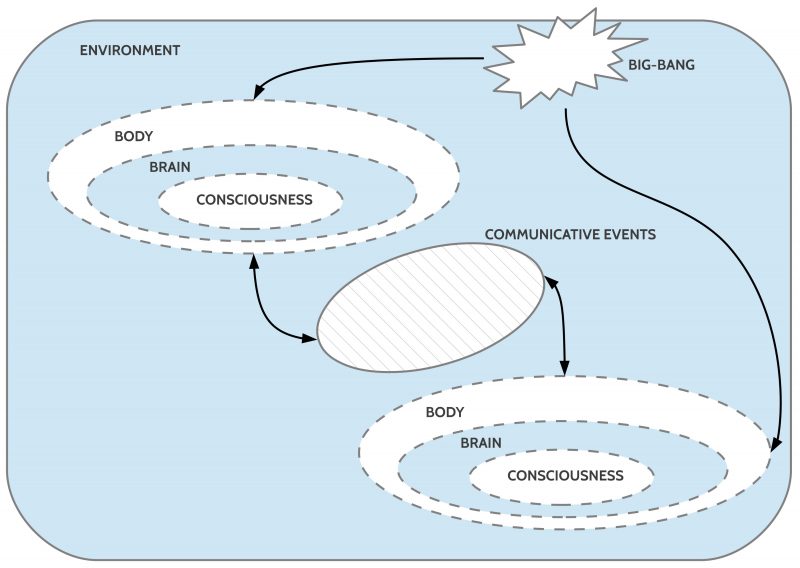
As the default standard case of an actor it is assumed that there are biological actors, usually human persons, which will not be analyzed with their inner structure [IS]. While the behavior of every system — and  therefore any biological system too — can be described with a behavior function φ: I x IS —> IS x O (if one has all the necessary knowledge), in the default case of biological systems  no behavior function φ is specified, φ = 0. During interactive simulations biological systems act by themselves.

If non-biological actors are used — e.g. automata with a certain machine program (an algorithm) — then one can use these only if one has a fully specified behavior function φ. From this follows that a  change rule which is associated with a non-biological actor has in its Eplus and in its Eminus part not a concrete expression but a variable, which will be computed during the simulation by the non-biological actor depending from its input and its behavior function φ: φ(input)IS=(Eplus, Eminus)IS.

FINAL COMMENT

Everybody who has read the parts (1) – (4) has now a general knowledge about the motivation to develop the oksimo software tool to support human kind to have a better communication and thinking of possible futures and a first understanding (hopefully :-)) how this tool can work. Reading the UN sustainable development goals [SDGs] [1] you will learn, that the SDG4 (Ensure inclusive and equitable quality education and promote lifelong learning opportunities for all) is fundamental to all other SDGs. The oksimo software tool is one tool to be of help to reach these goals.

REFERENCES

[1] The 2030 Agenda for Sustainable Development, adopted by all United Nations Member States in 2015, provides a shared blueprint for peace and prosperity for people and the planet, now and into the future. At its heart are the 17 Sustainable Development Goals (SDGs), which are an urgent call for action by all countries – developed and developing – in a global partnership. They recognize that ending poverty and other deprivations must go hand-in-hand with strategies that improve health and education, reduce inequality, and spur economic growth – all while tackling climate change and working to preserve our oceans and forests. See PDF: https://sdgs.un.org/sites/default/files/publication/21252030%20Agenda%20for%20Sustainable%20Development%20web.pdf

[2] UN, SDG4, PDF, Argumentation why the SDG4 ist fundamental for all other SDGs: https://sdgs.un.org/sites/default/files/publications/2275sdbeginswitheducation.pdf


STARTING WITH PYTHON3 – The very beginning – part 9

Journal: uffmm.org,
ISSN 2567-6458, July 24-25, 2019
Email: info@uffmm.org
Author: Gerd Doeben-Henisch
Email:gerd@doeben-henisch.de

CONTEXT

This is the next step in the python3 programming project. The overall context is still the python Co-Learning project.

SUBJECT

In this file you will see a first encounter between the AAI paradigm (described in the theory part of this uffmm blog) and some applications of the python programming language. A simple virtual world with objects and actors can become activated with a free selectable size, amount of objects and amount of actors. In later post lots of experiments with this virtual world will be described as well as many extensions.

SOURCE CODE
Main file: vw4.py

The main file ‘vw4.py’ describes the start of a virtual world and then allows a loop to run this world n-many times.

Import file: vwmanager.py

The main file ‘vw4.py’ is using many functions to enable the process. All these functions are collected in the file ‘vwmanager.py’. This file will automatically be loaded during run time of the program vw4.py.

COMMENTS

comment-vw4

DEMO

TEST RUN AUG 19, 2919, 12:56h

gerd@Doeben-Henisch:~/code$ python3 vw4.py
Amount of information: 1 is maximum, 0 is minimum0
Number of columns (= equal to rows!) of 2D-grid ?4
[‘_’, ‘_’, ‘_’, ‘_’]

[‘_’, ‘_’, ‘_’, ‘_’]

[‘_’, ‘_’, ‘_’, ‘_’]

[‘_’, ‘_’, ‘_’, ‘_’]

Percentage (as integer) of obstacles in the 2D-grid?77
Percentage (as integer) of Food Objects in the 2D-grid ?44
Percentage (as integer) of Actor Objects in the 2D-grid ?15

Objects as obstacles

[0, 2, ‘O’]

[0, 3, ‘O’]

[1, 2, ‘O’]

[2, 3, ‘O’]

Objects as food

[0, 0, ‘F’, [0, 1000, 100]]

[1, 1, ‘F’, [1, 1000, 100]]

[2, 0, ‘F’, [2, 1000, 100]]

[2, 2, ‘F’, [3, 1000, 100]]

[3, 0, ‘F’, [4, 1000, 100]]

[3, 3, ‘F’, [5, 1000, 100]]

Objects as actor

[1, 3, ‘A’, [0, 1000, 100, 500, 0]]

[3, 2, ‘A’, [1, 1000, 100, 500, 0]]

[‘F’, ‘_’, ‘O’, ‘O’]

[‘_’, ‘F’, ‘O’, ‘A’]

[‘F’, ‘_’, ‘F’, ‘O’]

[‘F’, ‘_’, ‘A’, ‘F’]

END OF PREPARATION

WORLD CYCLE STARTS

—————————————————-
Real percentage of obstacles = 25.0
Real percentage of food = 37.5
Real percentage of actors = 12.5
—————————————————-
How many CYCLES do you want?25
Singe Step = 1 or Continous = 0?1
Length of olA 2

—————————————————–

WORLD AT CYCLE = 0

[‘F’, ‘_’, ‘O’, ‘O’]

[‘_’, ‘F’, ‘O’, ‘A’]

[‘F’, ‘_’, ‘F’, ‘O’]

[‘F’, ‘_’, ‘A’, ‘F’]

Press key c for continuation!c
EEEEEEEEEEEEEEEEEEEEEEEEEEEEEEEEEEEEEEEEEEEEEEEEEEEEE

Updated energy levels in olF and olA
[1, 3, ‘A’, [0, 1000, 100, 500, -1]]

[2, 1, ‘A’, [1, 1000, 100, 500, 8]]

[0, 0, ‘F’, [0, 1000, 100]]

[1, 1, ‘F’, [1, 1000, 100]]

[2, 0, ‘F’, [2, 1000, 100]]

[2, 2, ‘F’, [3, 1000, 100]]

[3, 0, ‘F’, [4, 1000, 100]]

[3, 3, ‘F’, [5, 1000, 100]]

Length of olA 2

—————————————————–

WORLD AT CYCLE = 1

[‘F’, ‘_’, ‘O’, ‘O’]

[‘_’, ‘F’, ‘O’, ‘A’]

[‘F’, ‘A’, ‘F’, ‘O’]

[‘F’, ‘_’, ‘_’, ‘F’]

Press key c for continuation!c
EEEEEEEEEEEEEEEEEEEEEEEEEEEEEEEEEEEEEEEEEEEEEEEEEEEEE

Updated energy levels in olF and olA
[1, 3, ‘A’, [0, 900, 100, 500, -1]]

[2, 1, ‘A’, [1, 900, 100, 500, 0]]

[0, 0, ‘F’, [0, 1000, 100]]

[1, 1, ‘F’, [1, 1000, 100]]

[2, 0, ‘F’, [2, 1000, 100]]

[2, 2, ‘F’, [3, 1000, 100]]

[3, 0, ‘F’, [4, 1000, 100]]

[3, 3, ‘F’, [5, 1000, 100]]

Length of olA 2

—————————————————–

WORLD AT CYCLE = 2

[‘F’, ‘_’, ‘O’, ‘O’]

[‘_’, ‘F’, ‘O’, ‘A’]

[‘F’, ‘A’, ‘F’, ‘O’]

[‘F’, ‘_’, ‘_’, ‘F’]

Press key c for continuation!c
EEEEEEEEEEEEEEEEEEEEEEEEEEEEEEEEEEEEEEEEEEEEEEEEEEEEE

Updated energy levels in olF and olA
[1, 3, ‘A’, [0, 800, 100, 500, -1]]

[1, 1, ‘A’, [1, 1300, 100, 500, 1]]

[0, 0, ‘F’, [0, 1000, 100]]

[1, 1, ‘F’, [1, 500, 100]]

[2, 0, ‘F’, [2, 1000, 100]]

[2, 2, ‘F’, [3, 1000, 100]]

[3, 0, ‘F’, [4, 1000, 100]]

[3, 3, ‘F’, [5, 1000, 100]]

Length of olA 2

—————————————————–

WORLD AT CYCLE = 3

[‘F’, ‘_’, ‘O’, ‘O’]

[‘_’, ‘A’, ‘O’, ‘A’]

[‘F’, ‘_’, ‘F’, ‘O’]

[‘F’, ‘_’, ‘_’, ‘F’]

Press key c for continuation!c
EEEEEEEEEEEEEEEEEEEEEEEEEEEEEEEEEEEEEEEEEEEEEEEEEEEEE

Updated energy levels in olF and olA
[1, 3, ‘A’, [0, 700, 100, 500, -1]]

[2, 0, ‘A’, [1, 1700, 100, 500, 6]]

[0, 0, ‘F’, [0, 1000, 100]]

[1, 1, ‘F’, [1, 600, 100]]

[2, 0, ‘F’, [2, 500, 100]]

[2, 2, ‘F’, [3, 1000, 100]]

[3, 0, ‘F’, [4, 1000, 100]]

[3, 3, ‘F’, [5, 1000, 100]]

Length of olA 2

—————————————————–

WORLD AT CYCLE = 4

[‘F’, ‘_’, ‘O’, ‘O’]

[‘_’, ‘F’, ‘O’, ‘A’]

[‘A’, ‘_’, ‘F’, ‘O’]

[‘F’, ‘_’, ‘_’, ‘F’]

Press key c for continuation!c
EEEEEEEEEEEEEEEEEEEEEEEEEEEEEEEEEEEEEEEEEEEEEEEEEEEEE

Updated energy levels in olF and olA
[1, 3, ‘A’, [0, 600, 100, 500, -1]]

[1, 0, ‘A’, [1, 1600, 100, 500, 1]]

[0, 0, ‘F’, [0, 1000, 100]]

[1, 1, ‘F’, [1, 700, 100]]

[2, 0, ‘F’, [2, 600, 100]]

[2, 2, ‘F’, [3, 1000, 100]]

[3, 0, ‘F’, [4, 1000, 100]]

[3, 3, ‘F’, [5, 1000, 100]]

Length of olA 2

—————————————————–

WORLD AT CYCLE = 5

[‘F’, ‘_’, ‘O’, ‘O’]

[‘A’, ‘F’, ‘O’, ‘A’]

[‘F’, ‘_’, ‘F’, ‘O’]

[‘F’, ‘_’, ‘_’, ‘F’]

Press key c for continuation!c
EEEEEEEEEEEEEEEEEEEEEEEEEEEEEEEEEEEEEEEEEEEEEEEEEEEEE

Updated energy levels in olF and olA
[1, 3, ‘A’, [0, 500, 100, 500, -1]]

[1, 1, ‘A’, [1, 2000, 100, 500, 3]]

[0, 0, ‘F’, [0, 1000, 100]]

[1, 1, ‘F’, [1, 300, 100]]

[2, 0, ‘F’, [2, 700, 100]]

[2, 2, ‘F’, [3, 1000, 100]]

[3, 0, ‘F’, [4, 1000, 100]]

[3, 3, ‘F’, [5, 1000, 100]]

Length of olA 2

—————————————————–

WORLD AT CYCLE = 6

[‘F’, ‘_’, ‘O’, ‘O’]

[‘_’, ‘A’, ‘O’, ‘A’]

[‘F’, ‘_’, ‘F’, ‘O’]

[‘F’, ‘_’, ‘_’, ‘F’]

Press key c for continuation!c
EEEEEEEEEEEEEEEEEEEEEEEEEEEEEEEEEEEEEEEEEEEEEEEEEEEEE

Updated energy levels in olF and olA
[1, 3, ‘A’, [0, 400, 100, 500, -1]]

[1, 1, ‘A’, [1, 1900, 100, 500, -1]]

[0, 0, ‘F’, [0, 1000, 100]]

[1, 1, ‘F’, [1, 400, 100]]

[2, 0, ‘F’, [2, 800, 100]]

[2, 2, ‘F’, [3, 1000, 100]]

[3, 0, ‘F’, [4, 1000, 100]]

[3, 3, ‘F’, [5, 1000, 100]]

Length of olA 2

—————————————————–

WORLD AT CYCLE = 7

[‘F’, ‘_’, ‘O’, ‘O’]

[‘_’, ‘A’, ‘O’, ‘A’]

[‘F’, ‘_’, ‘F’, ‘O’]

[‘F’, ‘_’, ‘_’, ‘F’]

Press key c for continuation!c
EEEEEEEEEEEEEEEEEEEEEEEEEEEEEEEEEEEEEEEEEEEEEEEEEEEEE

Updated energy levels in olF and olA
[1, 3, ‘A’, [0, 300, 100, 500, -1]]

[1, 1, ‘A’, [1, 1800, 100, 500, -1]]

[0, 0, ‘F’, [0, 1000, 100]]

[1, 1, ‘F’, [1, 500, 100]]

[2, 0, ‘F’, [2, 900, 100]]

[2, 2, ‘F’, [3, 1000, 100]]

[3, 0, ‘F’, [4, 1000, 100]]

[3, 3, ‘F’, [5, 1000, 100]]

Length of olA 2

—————————————————–

WORLD AT CYCLE = 8

[‘F’, ‘_’, ‘O’, ‘O’]

[‘_’, ‘A’, ‘O’, ‘A’]

[‘F’, ‘_’, ‘F’, ‘O’]

[‘F’, ‘_’, ‘_’, ‘F’]

Press key c for continuation!c
EEEEEEEEEEEEEEEEEEEEEEEEEEEEEEEEEEEEEEEEEEEEEEEEEEEEE

Updated energy levels in olF and olA
[1, 3, ‘A’, [0, 200, 100, 500, -1]]

[1, 1, ‘A’, [1, 1700, 100, 500, -1]]

[0, 0, ‘F’, [0, 1000, 100]]

[1, 1, ‘F’, [1, 600, 100]]

[2, 0, ‘F’, [2, 1000, 100]]

[2, 2, ‘F’, [3, 1000, 100]]

[3, 0, ‘F’, [4, 1000, 100]]

[3, 3, ‘F’, [5, 1000, 100]]

Length of olA 2

—————————————————–

WORLD AT CYCLE = 9

[‘F’, ‘_’, ‘O’, ‘O’]

[‘_’, ‘A’, ‘O’, ‘A’]

[‘F’, ‘_’, ‘F’, ‘O’]

[‘F’, ‘_’, ‘_’, ‘F’]

Press key c for continuation!c
EEEEEEEEEEEEEEEEEEEEEEEEEEEEEEEEEEEEEEEEEEEEEEEEEEEEE

Updated energy levels in olF and olA
[1, 3, ‘A’, [0, 100, 100, 500, 0]]

[1, 0, ‘A’, [1, 1600, 100, 500, 7]]

[0, 0, ‘F’, [0, 1000, 100]]

[1, 1, ‘F’, [1, 700, 100]]

[2, 0, ‘F’, [2, 1000, 100]]

[2, 2, ‘F’, [3, 1000, 100]]

[3, 0, ‘F’, [4, 1000, 100]]

[3, 3, ‘F’, [5, 1000, 100]]

Length of olA 1

—————————————————–

WORLD AT CYCLE = 10

[‘F’, ‘_’, ‘O’, ‘O’]

[‘A’, ‘F’, ‘O’, ‘_’]

[‘F’, ‘_’, ‘F’, ‘O’]

[‘F’, ‘_’, ‘_’, ‘F’]

Press key c for continuation!c
EEEEEEEEEEEEEEEEEEEEEEEEEEEEEEEEEEEEEEEEEEEEEEEEEEEEE

Updated energy levels in olF and olA
[1, 0, ‘A’, [1, 1500, 100, 500, -1]]

[0, 0, ‘F’, [0, 1000, 100]]

[1, 1, ‘F’, [1, 800, 100]]

[2, 0, ‘F’, [2, 1000, 100]]

[2, 2, ‘F’, [3, 1000, 100]]

[3, 0, ‘F’, [4, 1000, 100]]

[3, 3, ‘F’, [5, 1000, 100]]

Length of olA 1

—————————————————–

WORLD AT CYCLE = 11

[‘F’, ‘_’, ‘O’, ‘O’]

[‘A’, ‘F’, ‘O’, ‘_’]

[‘F’, ‘_’, ‘F’, ‘O’]

[‘F’, ‘_’, ‘_’, ‘F’]

Press key c for continuation!c
EEEEEEEEEEEEEEEEEEEEEEEEEEEEEEEEEEEEEEEEEEEEEEEEEEEEE

Updated energy levels in olF and olA
[1, 0, ‘A’, [1, 1400, 100, 500, -1]]

[0, 0, ‘F’, [0, 1000, 100]]

[1, 1, ‘F’, [1, 900, 100]]

[2, 0, ‘F’, [2, 1000, 100]]

[2, 2, ‘F’, [3, 1000, 100]]

[3, 0, ‘F’, [4, 1000, 100]]

[3, 3, ‘F’, [5, 1000, 100]]

Length of olA 1

—————————————————–

WORLD AT CYCLE = 12

[‘F’, ‘_’, ‘O’, ‘O’]

[‘A’, ‘F’, ‘O’, ‘_’]

[‘F’, ‘_’, ‘F’, ‘O’]

[‘F’, ‘_’, ‘_’, ‘F’]

Press key c for continuation!c
EEEEEEEEEEEEEEEEEEEEEEEEEEEEEEEEEEEEEEEEEEEEEEEEEEEEE

Updated energy levels in olF and olA
[1, 0, ‘A’, [1, 1300, 100, 500, -1]]

[0, 0, ‘F’, [0, 1000, 100]]

[1, 1, ‘F’, [1, 1000, 100]]

[2, 0, ‘F’, [2, 1000, 100]]

[2, 2, ‘F’, [3, 1000, 100]]

[3, 0, ‘F’, [4, 1000, 100]]

[3, 3, ‘F’, [5, 1000, 100]]

Length of olA 1

—————————————————–

WORLD AT CYCLE = 13

[‘F’, ‘_’, ‘O’, ‘O’]

[‘A’, ‘F’, ‘O’, ‘_’]

[‘F’, ‘_’, ‘F’, ‘O’]

[‘F’, ‘_’, ‘_’, ‘F’]

Press key c for continuation!c
EEEEEEEEEEEEEEEEEEEEEEEEEEEEEEEEEEEEEEEEEEEEEEEEEEEEE

Updated energy levels in olF and olA
[2, 0, ‘A’, [1, 1700, 100, 500, 5]]

[0, 0, ‘F’, [0, 1000, 100]]

[1, 1, ‘F’, [1, 1000, 100]]

[2, 0, ‘F’, [2, 500, 100]]

[2, 2, ‘F’, [3, 1000, 100]]

[3, 0, ‘F’, [4, 1000, 100]]

[3, 3, ‘F’, [5, 1000, 100]]

Length of olA 1

—————————————————–

WORLD AT CYCLE = 14

[‘F’, ‘_’, ‘O’, ‘O’]

[‘_’, ‘F’, ‘O’, ‘_’]

[‘A’, ‘_’, ‘F’, ‘O’]

[‘F’, ‘_’, ‘_’, ‘F’]

Press key c for continuation!c
EEEEEEEEEEEEEEEEEEEEEEEEEEEEEEEEEEEEEEEEEEEEEEEEEEEEE

Updated energy levels in olF and olA
[1, 1, ‘A’, [1, 2100, 100, 500, 2]]

[0, 0, ‘F’, [0, 1000, 100]]

[1, 1, ‘F’, [1, 500, 100]]

[2, 0, ‘F’, [2, 600, 100]]

[2, 2, ‘F’, [3, 1000, 100]]

[3, 0, ‘F’, [4, 1000, 100]]

[3, 3, ‘F’, [5, 1000, 100]]

Length of olA 1

—————————————————–

WORLD AT CYCLE = 15

[‘F’, ‘_’, ‘O’, ‘O’]

[‘_’, ‘A’, ‘O’, ‘_’]

[‘F’, ‘_’, ‘F’, ‘O’]

[‘F’, ‘_’, ‘_’, ‘F’]

Press key c for continuation!c
EEEEEEEEEEEEEEEEEEEEEEEEEEEEEEEEEEEEEEEEEEEEEEEEEEEEE

Updated energy levels in olF and olA
[0, 0, ‘A’, [1, 2500, 100, 500, 8]]

[0, 0, ‘F’, [0, 500, 100]]

[1, 1, ‘F’, [1, 600, 100]]

[2, 0, ‘F’, [2, 700, 100]]

[2, 2, ‘F’, [3, 1000, 100]]

[3, 0, ‘F’, [4, 1000, 100]]

[3, 3, ‘F’, [5, 1000, 100]]

Length of olA 1

—————————————————–

WORLD AT CYCLE = 16

[‘A’, ‘_’, ‘O’, ‘O’]

[‘_’, ‘F’, ‘O’, ‘_’]

[‘F’, ‘_’, ‘F’, ‘O’]

[‘F’, ‘_’, ‘_’, ‘F’]

Press key c for continuation!c
EEEEEEEEEEEEEEEEEEEEEEEEEEEEEEEEEEEEEEEEEEEEEEEEEEEEE

Updated energy levels in olF and olA
[0, 0, ‘A’, [1, 2400, 100, 500, -1]]

[0, 0, ‘F’, [0, 600, 100]]

[1, 1, ‘F’, [1, 700, 100]]

[2, 0, ‘F’, [2, 800, 100]]

[2, 2, ‘F’, [3, 1000, 100]]

[3, 0, ‘F’, [4, 1000, 100]]

[3, 3, ‘F’, [5, 1000, 100]]

Length of olA 1

—————————————————–

WORLD AT CYCLE = 17

[‘A’, ‘_’, ‘O’, ‘O’]

[‘_’, ‘F’, ‘O’, ‘_’]

[‘F’, ‘_’, ‘F’, ‘O’]

[‘F’, ‘_’, ‘_’, ‘F’]

Press key c for continuation!c
EEEEEEEEEEEEEEEEEEEEEEEEEEEEEEEEEEEEEEEEEEEEEEEEEEEEE

Updated energy levels in olF and olA
[0, 0, ‘A’, [1, 2300, 100, 500, -1]]

[0, 0, ‘F’, [0, 700, 100]]

[1, 1, ‘F’, [1, 800, 100]]

[2, 0, ‘F’, [2, 900, 100]]

[2, 2, ‘F’, [3, 1000, 100]]

[3, 0, ‘F’, [4, 1000, 100]]

[3, 3, ‘F’, [5, 1000, 100]]

Length of olA 1

—————————————————–

WORLD AT CYCLE = 18

[‘A’, ‘_’, ‘O’, ‘O’]

[‘_’, ‘F’, ‘O’, ‘_’]

[‘F’, ‘_’, ‘F’, ‘O’]

[‘F’, ‘_’, ‘_’, ‘F’]

Press key c for continuation!c
EEEEEEEEEEEEEEEEEEEEEEEEEEEEEEEEEEEEEEEEEEEEEEEEEEEEE

Updated energy levels in olF and olA
[0, 0, ‘A’, [1, 2200, 100, 500, -1]]

[0, 0, ‘F’, [0, 800, 100]]

[1, 1, ‘F’, [1, 900, 100]]

[2, 0, ‘F’, [2, 1000, 100]]

[2, 2, ‘F’, [3, 1000, 100]]

[3, 0, ‘F’, [4, 1000, 100]]

[3, 3, ‘F’, [5, 1000, 100]]

Length of olA 1

—————————————————–

WORLD AT CYCLE = 19

[‘A’, ‘_’, ‘O’, ‘O’]

[‘_’, ‘F’, ‘O’, ‘_’]

[‘F’, ‘_’, ‘F’, ‘O’]

[‘F’, ‘_’, ‘_’, ‘F’]

Press key c for continuation!c
EEEEEEEEEEEEEEEEEEEEEEEEEEEEEEEEEEEEEEEEEEEEEEEEEEEEE

Updated energy levels in olF and olA
[0, 0, ‘A’, [1, 2100, 100, 500, -1]]

[0, 0, ‘F’, [0, 900, 100]]

[1, 1, ‘F’, [1, 1000, 100]]

[2, 0, ‘F’, [2, 1000, 100]]

[2, 2, ‘F’, [3, 1000, 100]]

[3, 0, ‘F’, [4, 1000, 100]]

[3, 3, ‘F’, [5, 1000, 100]]

Length of olA 1

—————————————————–

WORLD AT CYCLE = 20

[‘A’, ‘_’, ‘O’, ‘O’]

[‘_’, ‘F’, ‘O’, ‘_’]

[‘F’, ‘_’, ‘F’, ‘O’]

[‘F’, ‘_’, ‘_’, ‘F’]

Press key c for continuation!c
EEEEEEEEEEEEEEEEEEEEEEEEEEEEEEEEEEEEEEEEEEEEEEEEEEEEE

Updated energy levels in olF and olA
[0, 0, ‘A’, [1, 2000, 100, 500, -1]]

[0, 0, ‘F’, [0, 1000, 100]]

[1, 1, ‘F’, [1, 1000, 100]]

[2, 0, ‘F’, [2, 1000, 100]]

[2, 2, ‘F’, [3, 1000, 100]]

[3, 0, ‘F’, [4, 1000, 100]]

[3, 3, ‘F’, [5, 1000, 100]]

Length of olA 1

—————————————————–

WORLD AT CYCLE = 21

[‘A’, ‘_’, ‘O’, ‘O’]

[‘_’, ‘F’, ‘O’, ‘_’]

[‘F’, ‘_’, ‘F’, ‘O’]

[‘F’, ‘_’, ‘_’, ‘F’]

Press key c for continuation!c
EEEEEEEEEEEEEEEEEEEEEEEEEEEEEEEEEEEEEEEEEEEEEEEEEEEEE

Updated energy levels in olF and olA
[0, 0, ‘A’, [1, 1900, 100, 500, 0]]

[0, 0, ‘F’, [0, 1000, 100]]

[1, 1, ‘F’, [1, 1000, 100]]

[2, 0, ‘F’, [2, 1000, 100]]

[2, 2, ‘F’, [3, 1000, 100]]

[3, 0, ‘F’, [4, 1000, 100]]

[3, 3, ‘F’, [5, 1000, 100]]

Length of olA 1

—————————————————–

WORLD AT CYCLE = 22

[‘A’, ‘_’, ‘O’, ‘O’]

[‘_’, ‘F’, ‘O’, ‘_’]

[‘F’, ‘_’, ‘F’, ‘O’]

[‘F’, ‘_’, ‘_’, ‘F’]

Press key c for continuation!c
EEEEEEEEEEEEEEEEEEEEEEEEEEEEEEEEEEEEEEEEEEEEEEEEEEEEE

Updated energy levels in olF and olA
[0, 1, ‘A’, [1, 1800, 100, 500, 3]]

[0, 0, ‘F’, [0, 1000, 100]]

[1, 1, ‘F’, [1, 1000, 100]]

[2, 0, ‘F’, [2, 1000, 100]]

[2, 2, ‘F’, [3, 1000, 100]]

[3, 0, ‘F’, [4, 1000, 100]]

[3, 3, ‘F’, [5, 1000, 100]]

Length of olA 1

—————————————————–

WORLD AT CYCLE = 23

[‘F’, ‘A’, ‘O’, ‘O’]

[‘_’, ‘F’, ‘O’, ‘_’]

[‘F’, ‘_’, ‘F’, ‘O’]

[‘F’, ‘_’, ‘_’, ‘F’]

Press key c for continuation!c
EEEEEEEEEEEEEEEEEEEEEEEEEEEEEEEEEEEEEEEEEEEEEEEEEEEEE

Updated energy levels in olF and olA
[1, 1, ‘A’, [1, 2200, 100, 500, 5]]

[0, 0, ‘F’, [0, 1000, 100]]

[1, 1, ‘F’, [1, 500, 100]]

[2, 0, ‘F’, [2, 1000, 100]]

[2, 2, ‘F’, [3, 1000, 100]]

[3, 0, ‘F’, [4, 1000, 100]]

[3, 3, ‘F’, [5, 1000, 100]]

Length of olA 1

—————————————————–

WORLD AT CYCLE = 24

[‘F’, ‘_’, ‘O’, ‘O’]

[‘_’, ‘A’, ‘O’, ‘_’]

[‘F’, ‘_’, ‘F’, ‘O’]

[‘F’, ‘_’, ‘_’, ‘F’]

Press key c for continuation!c
EEEEEEEEEEEEEEEEEEEEEEEEEEEEEEEEEEEEEEEEEEEEEEEEEEEEE

Updated energy levels in olF and olA
[1, 1, ‘A’, [1, 2100, 100, 500, -1]]

[0, 0, ‘F’, [0, 1000, 100]]

[1, 1, ‘F’, [1, 600, 100]]

[2, 0, ‘F’, [2, 1000, 100]]

[2, 2, ‘F’, [3, 1000, 100]]

[3, 0, ‘F’, [4, 1000, 100]]

[3, 3, ‘F’, [5, 1000, 100]]


AAI THEORY V2 –A Philosophical Framework

eJournal: uffmm.org,
ISSN 2567-6458, 22.February 2019
Email: info@uffmm.org
Author: Gerd Doeben-Henisch
Email: gerd@doeben-henisch.de

Last change: 23.February 2019 (continued the text)

Last change: 24.February 2019 (extended the text)

CONTEXT

In the overview of the AAI paradigm version 2 you can find this section  dealing with the philosophical perspective of the AAI paradigm. Enjoy reading (or not, then send a comment :-)).

THE DAILY LIFE PERSPECTIVE

The perspective of Philosophy is rooted in the everyday life perspective. With our body we occur in a space with other bodies and objects; different features, properties  are associated with the objects, different kinds of relations an changes from one state to another.

From the empirical sciences we have learned to see more details of the everyday life with regard to detailed structures of matter and biological life, with regard to the long history of the actual world, with regard to many interesting dynamics within the objects, within biological systems, as part of earth, the solar system and much more.

A certain aspect of the empirical view of the world is the fact, that some biological systems called ‘homo sapiens’, which emerged only some 300.000 years ago in Africa, show a special property usually called ‘consciousness’ combined with the ability to ‘communicate by symbolic languages’.

General setting of the homo sapiens species (simplified)
Figure 1: General setting of the homo sapiens species (simplified)

As we know today the consciousness is associated with the brain, which in turn is embedded in the body, which  is further embedded in an environment.

Thus those ‘things’ about which we are ‘conscious’ are not ‘directly’ the objects and events of the surrounding real world but the ‘constructions of the brain’ based on actual external and internal sensor inputs as well as already collected ‘knowledge’. To qualify the ‘conscious things’ as ‘different’ from the assumed ‘real things’ ‘outside there’ it is common to speak of these brain-generated virtual things either as ‘qualia’ or — more often — as ‘phenomena’ which are  different to the assumed possible real things somewhere ‘out there’.

PHILOSOPHY AS FIRST PERSON VIEW

‘Philosophy’ has many facets.  One enters the scene if we are taking the insight into the general virtual character of our primary knowledge to be the primary and irreducible perspective of knowledge.  Every other more special kind of knowledge is necessarily a subspace of this primary phenomenological knowledge.

There is already from the beginning a fundamental distinction possible in the realm of conscious phenomena (PH): there are phenomena which can be ‘generated’ by the consciousness ‘itself’  — mostly called ‘by will’ — and those which are occurring and disappearing without a direct influence of the consciousness, which are in a certain basic sense ‘given’ and ‘independent’,  which are appearing  and disappearing according to ‘their own’. It is common to call these independent phenomena ’empirical phenomena’ which represent a true subset of all phenomena: PH_emp  PH. Attention: These empirical phenomena’ are still ‘phenomena’, virtual entities generated by the brain inside the brain, not directly controllable ‘by will’.

There is a further basic distinction which differentiates the empirical phenomena into those PH_emp_bdy which are controlled by some processes in the body (being tired, being hungry, having pain, …) and those PH_emp_ext which are controlled by objects and events in the environment beyond the body (light, sounds, temperature, surfaces of objects, …). Both subsets of empirical phenomena are different: PH_emp_bdy PH_emp_ext = 0. Because phenomena usually are occurring  associated with typical other phenomena there are ‘clusters’/ ‘pattern’ of phenomena which ‘represent’ possible events or states.

Modern empirical science has ‘refined’ the concept of an empirical phenomenon by introducing  ‘standard objects’ which can be used to ‘compare’ some empirical phenomenon with such an empirical standard object. Thus even when the perception of two different observers possibly differs somehow with regard to a certain empirical phenomenon, the additional comparison with an ’empirical standard object’ which is the ‘same’ for both observers, enhances the quality, improves the precision of the perception of the empirical phenomena.

From these considerations we can derive the following informal definitions:

  1. Something is ‘empirical‘ if it is the ‘real counterpart’ of a phenomenon which can be observed by other persons in my environment too.
  2. Something is ‘standardized empirical‘ if it is empirical and can additionally be associated with a before introduced empirical standard object.
  3. Something is ‘weak empirical‘ if it is the ‘real counterpart’ of a phenomenon which can potentially be observed by other persons in my body as causally correlated with the phenomenon.
  4. Something is ‘cognitive‘ if it is the counterpart of a phenomenon which is not empirical in one of the meanings (1) – (3).

It is a common task within philosophy to analyze the space of the phenomena with regard to its structure as well as to its dynamics.  Until today there exists not yet a complete accepted theory for this subject. This indicates that this seems to be some ‘hard’ task to do.

BRIDGING THE GAP BETWEEN BRAINS

As one can see in figure 1 a brain in a body is completely disconnected from the brain in another body. There is a real, deep ‘gap’ which has to be overcome if the two brains want to ‘coordinate’ their ‘planned actions’.

Luckily the emergence of homo sapiens with the new extended property of ‘consciousness’ was accompanied by another exciting property, the ability to ‘talk’. This ability enabled the creation of symbolic languages which can help two disconnected brains to have some exchange.

But ‘language’ does not consist of sounds or a ‘sequence of sounds’ only; the special power of a language is the further property that sequences of sounds can be associated with ‘something else’ which serves as the ‘meaning’ of these sounds. Thus we can use sounds to ‘talk about’ other things like objects, events, properties etc.

The single brain ‘knows’ about the relationship between some sounds and ‘something else’ because the brain is able to ‘generate relations’ between brain-structures for sounds and brain-structures for something else. These relations are some real connections in the brain. Therefore sounds can be related to ‘something  else’ or certain objects, and events, objects etc.  can become related to certain sounds. But these ‘meaning relations’ can only ‘bridge the gap’ to another brain if both brains are using the same ‘mapping’, the same ‘encoding’. This is only possible if the two brains with their bodies share a real world situation RW_S where the perceptions of the both brains are associated with the same parts of the real world between both bodies. If this is the case the perceptions P(RW_S) can become somehow ‘synchronized’ by the shared part of the real world which in turn is transformed in the brain structures P(RW_S) —> B_S which represent in the brain the stimulating aspects of the real world.  These brain structures B_S can then be associated with some sound structures B_A written as a relation  MEANING(B_S, B_A). Such a relation  realizes an encoding which can be used for communication. Communication is using sound sequences exchanged between brains via the body and the air of an environment as ‘expressions’ which can be recognized as part of a learned encoding which enables the receiving brain to identify a possible meaning candidate.

DIFFERENT MODES TO EXPRESS MEANING

Following the evolution of communication one can distinguish four important modes of expressing meaning, which will be used in this AAI paradigm.

VISUAL ENCODING

A direct way to express the internal meaning structures of a brain is to use a ‘visual code’ which represents by some kinds of drawing the visual shapes of objects in the space, some attributes of  shapes, which are common for all people who can ‘see’. Thus a picture and then a sequence of pictures like a comic or a story board can communicate simple ideas of situations, participating objects, persons and animals, showing changes in the arrangement of the shapes in the space.

Pictorial expressions representing aspects of the visual and the auditory sens modes
Figure 2: Pictorial expressions representing aspects of the visual and the auditory sens modes

Even with a simple visual code one can generate many sequences of situations which all together can ‘tell a story’. The basic elements are a presupposed ‘space’ with possible ‘objects’ in this space with different positions, sizes, relations and properties. One can even enhance these visual shapes with written expressions of  a spoken language. The sequence of the pictures represents additionally some ‘timely order’. ‘Changes’ can be encoded by ‘differences’ between consecutive pictures.

FROM SPOKEN TO WRITTEN LANGUAGE EXPRESSIONS

Later in the evolution of language, much later, the homo sapiens has learned to translate the spoken language L_s in a written format L_w using signs for parts of words or even whole words.  The possible meaning of these written expressions were no longer directly ‘visible’. The meaning was now only available for those people who had learned how these written expressions are associated with intended meanings encoded in the head of all language participants. Thus only hearing or reading a language expression would tell the reader either ‘nothing’ or some ‘possible meanings’ or a ‘definite meaning’.

A written textual version in parallel to a pictorial version
Figure 3: A written textual version in parallel to a pictorial version

If one has only the written expressions then one has to ‘know’ with which ‘meaning in the brain’ the expressions have to be associated. And what is very special with the written expressions compared to the pictorial expressions is the fact that the elements of the pictorial expressions are always very ‘concrete’ visual objects while the written expressions are ‘general’ expressions allowing many different concrete interpretations. Thus the expression ‘person’ can be used to be associated with many thousands different concrete objects; the same holds for the expression ‘road’, ‘moving’, ‘before’ and so on. Thus the written expressions are like ‘manufacturing instructions’ to search for possible meanings and configure these meanings to a ‘reasonable’ complex matter. And because written expressions are in general rather ‘abstract’/ ‘general’ which allow numerous possible concrete realizations they are very ‘economic’ because they use minimal expressions to built many complex meanings. Nevertheless the daily experience with spoken and written expressions shows that they are continuously candidates for false interpretations.

FORMAL MATHEMATICAL WRITTEN EXPRESSIONS

Besides the written expressions of everyday languages one can observe later in the history of written languages the steady development of a specialized version called ‘formal languages’ L_f with many different domains of application. Here I am  focusing   on the formal written languages which are used in mathematics as well as some pictorial elements to ‘visualize’  the intended ‘meaning’ of these formal mathematical expressions.

Properties of an acyclic directed graph with nodes (vertices) and edges (directed edges = arrows)
Fig. 4: Properties of an acyclic directed graph with nodes (vertices) and edges (directed edges = arrows)

One prominent concept in mathematics is the concept of a ‘graph’. In  the basic version there are only some ‘nodes’ (also called vertices) and some ‘edges’ connecting the nodes.  Formally one can represent these edges as ‘pairs of nodes’. If N represents the set of nodes then N x N represents the set of all pairs of these nodes.

In a more specialized version the edges are ‘directed’ (like a ‘one way road’) and also can be ‘looped back’ to a node   occurring ‘earlier’ in the graph. If such back-looping arrows occur a graph is called a ‘cyclic graph’.

Directed cyclic graph extended to represent 'states of affairs'
Fig.5: Directed cyclic graph extended to represent ‘states of affairs’

If one wants to use such a graph to describe some ‘states of affairs’ with their possible ‘changes’ one can ‘interpret’ a ‘node’ as  a state of affairs and an arrow as a change which turns one state of affairs S in a new one S’ which is minimally different to the old one.

As a state of affairs I  understand here a ‘situation’ embedded in some ‘context’ presupposing some common ‘space’. The possible ‘changes’ represented by arrows presuppose some dimension of ‘time’. Thus if a node n’  is following a node n indicated by an arrow then the state of affairs represented by the node n’ is to interpret as following the state of affairs represented in the node n with regard to the presupposed time T ‘later’, or n < n’ with ‘<‘ as a symbol for a timely ordering relation.

Example of a state of affairs with a 2-dimensional space configured as a grid with a black and a white token
Fig.6: Example of a state of affairs with a 2-dimensional space configured as a grid with a black and a white token

The space can be any kind of a space. If one assumes as an example a 2-dimensional space configured as a grid –as shown in figure 6 — with two tokens at certain positions one can introduce a language to describe the ‘facts’ which constitute the state of affairs. In this example one needs ‘names for objects’, ‘properties of objects’ as well as ‘relations between objects’. A possible finite set of facts for situation 1 could be the following:

  1. TOKEN(T1), BLACK(T1), POSITION(T1,1,1)
  2. TOKEN(T2), WHITE(T2), POSITION(T2,2,1)
  3. NEIGHBOR(T1,T2)
  4. CELL(C1), POSITION(1,2), FREE(C1)

‘T1’, ‘T2’, as well as ‘C1’ are names of objects, ‘TOKEN’, ‘BACK’ etc. are names of properties, and ‘NEIGHBOR’ is a relation between objects. This results in the equation:

S1 = {TOKEN(T1), BLACK(T1), POSITION(T1,1,1), TOKEN(T2), WHITE(T2), POSITION(T2,2,1), NEIGHBOR(T1,T2), CELL(C1), POSITION(1,2), FREE(C1)}

These facts describe the situation S1. If it is important to describe possible objects ‘external to the situation’ as important factors which can cause some changes then one can describe these objects as a set of facts  in a separated ‘context’. In this example this could be two players which can move the black and white tokens and thereby causing a change of the situation. What is the situation and what belongs to a context is somewhat arbitrary. If one describes the agriculture of some region one usually would not count the planets and the atmosphere as part of this region but one knows that e.g. the sun can severely influence the situation   in combination with the atmosphere.

Change of a state of affairs given as a state which will be enhanced by a new object
Fig.7: Change of a state of affairs given as a state which will be enhanced by a new object

Let us stay with a state of affairs with only a situation without a context. The state of affairs is     a ‘state’. In the example shown in figure 6 I assume a ‘change’ caused by the insertion of a new black token at position (2,2). Written in the language of facts L_fact we get:

  1. TOKEN(T3), BLACK(T3), POSITION(2,2), NEIGHBOR(T3,T2)

Thus the new state S2 is generated out of the old state S1 by unifying S1 with the set of new facts: S2 = S1 {TOKEN(T3), BLACK(T3), POSITION(2,2), NEIGHBOR(T3,T2)}. All the other facts of S1 are still ‘valid’. In a more general manner one can introduce a change-expression with the following format:

<S1, S2, add(S1,{TOKEN(T3), BLACK(T3), POSITION(2,2), NEIGHBOR(T3,T2)})>

This can be read as follows: The follow-up state S2 is generated out of the state S1 by adding to the state S1 the set of facts { … }.

This layout of a change expression can also be used if some facts have to be modified or removed from a state. If for instance  by some reason the white token should be removed from the situation one could write:

<S1, S2, subtract(S1,{TOKEN(T2), WHITE(T2), POSITION(2,1)})>

Another notation for this is S2 = S1 – {TOKEN(T2), WHITE(T2), POSITION(2,1)}.

The resulting state S2 would then look like:

S2 = {TOKEN(T1), BLACK(T1), POSITION(T1,1,1), CELL(C1), POSITION(1,2), FREE(C1)}

And a combination of subtraction of facts and addition of facts would read as follows:

<S1, S2, subtract(S1,{TOKEN(T2), WHITE(T2), POSITION(2,1)}, add(S1,{TOKEN(T3), BLACK(T3), POSITION(2,2)})>

This would result in the final state S2:

S2 = {TOKEN(T1), BLACK(T1), POSITION(T1,1,1), CELL(C1), POSITION(1,2), FREE(C1),TOKEN(T3), BLACK(T3), POSITION(2,2)}

These simple examples demonstrate another fact: while facts about objects and their properties are independent from each other do relational facts depend from the state of their object facts. The relation of neighborhood e.g. depends from the participating neighbors. If — as in the example above — the object token T2 disappears then the relation ‘NEIGHBOR(T1,T2)’ no longer holds. This points to a hierarchy of dependencies with the ‘basic facts’ at the ‘root’ of a situation and all the other facts ‘above’ basic facts or ‘higher’ depending from the basic facts. Thus ‘higher order’ facts should be added only for the actual state and have to be ‘re-computed’ for every follow-up state anew.

If one would specify a context for state S1 saying that there are two players and one allows for each player actions like ‘move’, ‘insert’ or ‘delete’ then one could make the change from state S1 to state S2 more precise. Assuming the following facts for the context:

  1. PLAYER(PB1), PLAYER(PW1), HAS-THE-TURN(PB1)

In that case one could enhance the change statement in the following way:

<S1, S2, PB1,insert(TOKEN(T3,2,2)),add(S1,{TOKEN(T3), BLACK(T3), POSITION(2,2)})>

This would read as follows: given state S1 the player PB1 inserts a  black token at position (2,2); this yields a new state S2.

With or without a specified context but with regard to a set of possible change statements it can be — which is the usual case — that there is more than one option what can be changed. Some of the main types of changes are the following ones:

  1. RANDOM
  2. NOT RANDOM, which can be specified as follows:
    1. With PROBABILITIES (classical, quantum probability, …)
    2. DETERMINISTIC

Furthermore, if the causing object is an actor which can adapt structurally or even learn locally then this actor can appear in some time period like a deterministic system, in different collected time periods as an ‘oscillating system’ with different behavior, or even as a random system with changing probabilities. This make the forecast of systems with adaptive and/ or learning systems rather difficult.

Another aspect results from the fact that there can be states either with one actor which can cause more than one action in parallel or a state with multiple actors which can act simultaneously. In both cases the resulting total change has eventually to be ‘filtered’ through some additional rules telling what  is ‘possible’ in a state and what not. Thus if in the example of figure 6 both player want to insert a token at position (2,2) simultaneously then either  the rules of the game would forbid such a simultaneous action or — like in a computer game — simultaneous actions are allowed but the ‘geometry of a 2-dimensional space’ would not allow that two different tokens are at the same position.

Another aspect of change is the dimension of time. If the time dimension is not explicitly specified then a change from some state S_i to a state S_j does only mark the follow up state S_j as later. There is no specific ‘metric’ of time. If instead a certain ‘clock’ is specified then all changes have to be aligned with this ‘overall clock’. Then one can specify at what ‘point of time t’ the change will begin and at what point of time t*’ the change will be ended. If there is more than one change specified then these different changes can have different timings.

THIRD PERSON VIEW

Up until now the point of view describing a state and the possible changes of states is done in the so-called 3rd-person view: what can a person perceive if it is part of a situation and is looking into the situation.  It is explicitly assumed that such a person can perceive only the ‘surface’ of objects, including all kinds of actors. Thus if a driver of a car stears his car in a certain direction than the ‘observing person’ can see what happens, but can not ‘look into’ the driver ‘why’ he is steering in this way or ‘what he is planning next’.

A 3rd-person view is assumed to be the ‘normal mode of observation’ and it is the normal mode of empirical science.

Nevertheless there are situations where one wants to ‘understand’ a bit more ‘what is going on in a system’. Thus a biologist can be  interested to understand what mechanisms ‘inside a plant’ are responsible for the growth of a plant or for some kinds of plant-disfunctions. There are similar cases for to understand the behavior of animals and men. For instance it is an interesting question what kinds of ‘processes’ are in an animal available to ‘navigate’ in the environment across distances. Even if the biologist can look ‘into the body’, even ‘into the brain’, the cells as such do not tell a sufficient story. One has to understand the ‘functions’ which are enabled by the billions of cells, these functions are complex relations associated with certain ‘structures’ and certain ‘signals’. For this it is necessary to construct an explicit formal (mathematical) model/ theory representing all the necessary signals and relations which can be used to ‘explain’ the obsrvable behavior and which ‘explains’ the behavior of the billions of cells enabling such a behavior.

In a simpler, ‘relaxed’ kind of modeling  one would not take into account the properties and behavior of the ‘real cells’ but one would limit the scope to build a formal model which suffices to explain the oservable behavior.

This kind of approach to set up models of possible ‘internal’ (as such hidden) processes of an actor can extend the 3rd-person view substantially. These models are called in this text ‘actor models (AM)’.

HIDDEN WORLD PROCESSES

In this text all reported 3rd-person observations are called ‘actor story’, independent whether they are done in a pictorial or a textual mode.

As has been pointed out such actor stories are somewhat ‘limited’ in what they can describe.

It is possible to extend such an actor story (AS)  by several actor models (AM).

An actor story defines the situations in which an actor can occur. This  includes all kinds of stimuli which can trigger the possible senses of the actor as well as all kinds of actions an actor can apply to a situation.

The actor model of such an actor has to enable the actor to handle all these assumed stimuli as well as all these actions in the expected way.

While the actor story can be checked whether it is describing a process in an empirical ‘sound’ way,  the actor models are either ‘purely theoretical’ but ‘behavioral sound’ or they are also empirically sound with regard to the body of a biological or a technological system.

A serious challenge is the occurrence of adaptiv or/ and locally learning systems. While the actor story is a finite  description of possible states and changes, adaptiv or/ and locally learning systeme can change their behavior while ‘living’ in the actor story. These changes in the behavior can not completely be ‘foreseen’!

COGNITIVE EXPERT PROCESSES

According to the preceding considerations a homo sapiens as a biological system has besides many properties at least a consciousness and the ability to talk and by this to communicate with symbolic languages.

Looking to basic modes of an actor story (AS) one can infer some basic concepts inherently present in the communication.

Without having an explicit model of the internal processes in a homo sapiens system one can infer some basic properties from the communicative acts:

  1. Speaker and hearer presuppose a space within which objects with properties can occur.
  2. Changes can happen which presuppose some timely ordering.
  3. There is a disctinction between concrete things and abstract concepts which correspond to many concrete things.
  4. There is an implicit hierarchy of concepts starting with concrete objects at the ‘root level’ given as occurence in a concrete situation. Other concepts of ‘higher levels’ refer to concepts of lower levels.
  5. There are different kinds of relations between objects on different conceptual levels.
  6. The usage of language expressions presupposes structures which can be associated with the expressions as their ‘meanings’. The mapping between expressions and their meaning has to be learned by each actor separately, but in cooperation with all the other actors, with which the actor wants to share his meanings.
  7. It is assume that all the processes which enable the generation of concepts, concept hierarchies, relations, meaning relations etc. are unconscious! In the consciousness one can  use parts of the unconscious structures and processes under strictly limited conditions.
  8. To ‘learn’ dedicated matters and to be ‘critical’ about the quality of what one is learnig requires some disciplin, some learning methods, and a ‘learning-friendly’ environment. There is no guaranteed method of success.
  9. There are lots of unconscious processes which can influence understanding, learning, planning, decisions etc. and which until today are not yet sufficiently cleared up.


ADVANCED AAI-THEORY

eJournal: uffmm.org,
ISSN 2567-6458, 21.Januar 2019
Email: info@uffmm.org
Author: Gerd Doeben-Henisch
Email: gerd@doeben-henisch.de

Here You can find a new version of this post

CONTEXT

The last official update of the AAI theory dates back to Oct-2, 2018. Since that time many new thoughts have been detected and have been configured for further extensions and improvements. Here I try to give an overview of all the actual known aspects of the expanded AAI theory as a possible guide for the further elaborations of the main text.

CLARIFYING THE PROBLEM

  1. Generally it is assumed that the AAI theory is embedded in a general systems engineering approach starting with the clarification of a problem.
  2. Two cases will be distinguished:
    1. A stakeholder is associated with a certain domain of affairs with some prominent aspect/ parameter P and the stakeholder wants to clarify whether P poses some ‘problem’ in this domain. This presupposes some explained ‘expectations’ E how it should be and some ‘findings’ x pointing to the fact that P is ‘sufficiently different’ from some y>x. If the stakeholder judges that this difference is ‘important’, than P matching x will be classified as a problem, which will be documented in a ‘problem document D_p’. One interpret this this analysis as a ‘measurement M’ written as M(P,E) = x and x<y.
    2. Given a problem document D_p a stakeholder invites some experts to find a ‘solution’ which transfers the old ‘problem P’ into a ‘configuration S’ which at least should ‘minimize the problem P’. Thus there must exist some ‘measurements’ of the given problem P with regard to certain ‘expectations E’ functioning as a ‘norm’ as M(P,E)=x and some measurements of the new configuration S with regard to the same expectations E as M(S,E)=y and a metric which allows the judgment y > x.
  3. From this follows that already in the beginning of the analysis of a possible solution one has to refer to some measurement process M, otherwise there exists no problem P.

CHECK OF FRAMING CONDITIONS

  1. The definition of a problem P presupposes a domain of affairs which has to be characterized in at least two respects:
    1. A minimal description of an environment ENV of the problem P and
    2. a list of so-called non-functional requirements (NFRs).
  2. Within the environment it mus be possible to identify at least one task T to be realized from some start state to some end state.
  3. Additionally it mus be possible to identify at least one executing actor A_exec doing this task and at least one actor assisting A_ass the executing actor to fulfill the task.
  4. For the  following analysis of a possible solution one can distinguish two strategies:
    1. Top-down: There exists a group of experts EXPs which will analyze a possible solution, will test these, and then will propose these as a solution for others.
    2. Bottom-up: There exists a group of experts EXPs too but additionally there exists a group of customers CTMs which will be guided by the experts to use their own experience to find a possible solution.

ACTOR STORY (AS)

  1. The goal of an actor story (AS) is a full specification of all identified necessary tasks T which lead from a start state q* to a goal state q+, including all possible and necessary changes between the different states M.
  2. A state is here considered as a finite set of facts (F) which are structured as an expression from some language L distinguishing names of objects (LIKE ‘d1’, ‘u1’, …) as well as properties of objects (like ‘being open’, ‘being green’, …) or relations between objects (like ‘the user stands before the door’). There can also e a ‘negation’ like ‘the door is not open’. Thus a collection of facts like ‘There is a door D1’ and ‘The door D1 is open’ can represent a state.
  3. Changes from one state q to another successor state q’ are described by the object whose action deletes previous facts or creates new facts.
  4. In this approach at least three different modes of an actor story will be distinguished:
    1. A pictorial mode generating a Pictorial Actor Story (PAS). In a pictorial mode the drawings represent the main objects with their properties and relations in an explicit visual way (like a Comic Strip).
    2. A textual mode generating a Textual Actor Story (TAS): In a textual mode a text in some everyday language (e.g. in English) describes the states and changes in plain English. Because in the case of a written text the meaning of the symbols is hidden in the heads of the writers it can be of help to parallelize the written text with the pictorial mode.
    3. A mathematical mode generating a Mathematical Actor Story (MAS): n the mathematical mode the pictorial and the textual modes are translated into sets of formal expressions forming a graph whose nodes are sets of facts and whose edges are labeled with change-expressions.

TASK INDUCED ACTOR-REQUIREMENTS (TAR)

If an actor story AS is completed, then one can infer from this story all the requirements which are directed at the executing as well as the assistive actors of the story. These requirements are targeting the needed input- as well as output-behavior of the actors from a 3rd person point of view (e.g. what kinds of perception are required, what kinds of motor reactions, etc.).

ACTOR INDUCED ACTOR-REQUIREMENTS (AAR)

Depending from the kinds of actors planned for the real work (biological systems, animals or humans; machines, different kinds of robots), one has to analyze the required internal structures of the actors needed to enable the required perceptions and responses. This has to be done in a 1st person point of view.

ACTOR MODELS (AMs)

Based on the AARs one has to construct explicit actor models which are fulfilling the requirements.

USABILITY TESTING (UTST)

Using the actor as a ‘norm’ for the measurement one has to organized an ‘usability test’ in he way, that a real executing test actor having the required profiles has to use a real assisting actor in the context of the specified actor story. Place in a start state of the actor story the executing test actor has to show that and how he will reach the defined goal state of the actor story. For this he has to use a real assistive actor which usually is an experimental device (a mock-up), which allows the test of the story.

Because an executive actor is usually a ‘learning actor’ one has to repeat the usability test n-times to see, whether the learning curve approaches a minimum. Additionally to such objective tests one should also organize an interview to get some judgments about the subjective states of the test persons.

SIMULATION

With an increasing complexity of an actor story AS it becomes important to built a simulator (SIM) which can take as input the start state of the actor story together with all possible changes. Then the simulator can compute — beginning with the start state — all possible successor states. In the interactive mode participating actors will explicitly be asked to interact with the simulator.

Having a simulator one can use a simulator as part of an usability test to mimic the behavior of an assistive actor. This mode can also be used for training new executive actors.

A TOP-DOWN ACTOR STORY

The elaboration of an actor story will usually be realized in a top-down style: some AAI experts will develop the actor story based on their experience and will only ask for some test persons if they have elaborated everything so far that they can define some tests.

A BOTTOM-UP ACTOR STORY

In a bottom-up style the AAI experts collaborate from the beginning with a group of common users from the application domain. To do this they will (i) extract the knowledge which is distributed in the different users, then (ii) they will start some modeling from these different facts to (iii) enable some basic simulations. This simple simulation (iv) will be enhanced to an interactive simulation which allows serious gaming either (iv.a) to test the model or to enable the users (iv.b) to learn the space of possible states. The test case will (v) generate some data which can be used to evaluate the model with regard to pre-defined goals. Depending from these findings (vi) one can try to improve the model further.

THE COGNITIVE SPACE

To be able to construct executive as well as assistive actors which are close to the way how human persons do communicate one has to set up actor models which are as close as possible with the human style of cognition. This requires the analysis of phenomenal experience as well as the psychological behavior as well as the analysis of a needed neuron-physiological structures.

STATE DYNAMICS

To model in an actor story the possible changes from one given state to another one (or to many successor states) one needs eventually besides explicit deterministic changes different kinds of random rules together with adaptive ones or decision-based behavior depending from a whole network of changing parameters.