Journal: uffmm.org,
ISSN 2567-6458, July 24-25, 2019
Email: info@uffmm.org
Author: Gerd Doeben-Henisch
Email:gerd@doeben-henisch.de
CONTEXT
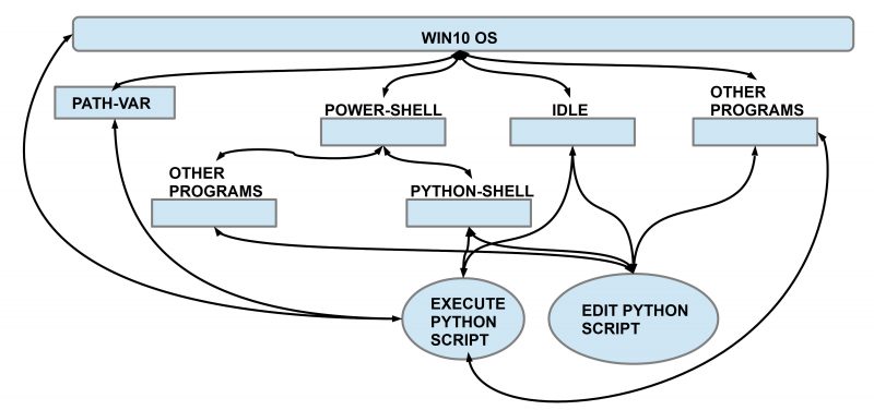
This is the next step in the python3 programming project. The overall context is still the python Co-Learning project.
SUBJECT
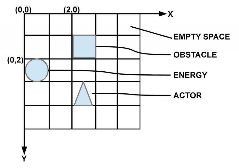
In this file you will see a first encounter between the AAI paradigm (described in the theory part of this uffmm blog) and some applications of the python programming language. A simple virtual world with objects and actors can become activated with a free selectable size, amount of objects and amount of actors. In later post lots of experiments with this virtual world will be described as well as many extensions.
SOURCE CODE
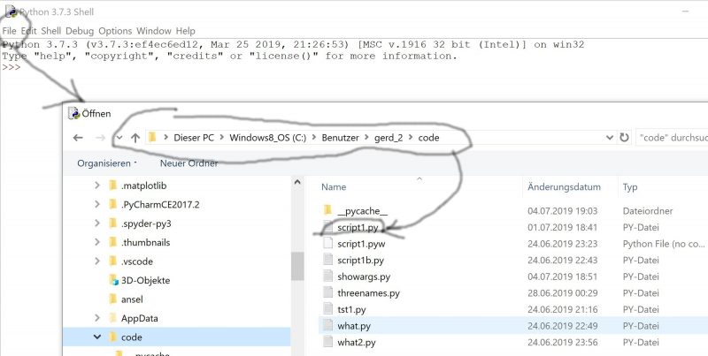
The main file ‘vw4.py’ describes the start of a virtual world and then allows a loop to run this world n-many times.
The main file ‘vw4.py’ is using many functions to enable the process. All these functions are collected in the file ‘vwmanager.py’. This file will automatically be loaded during run time of the program vw4.py.
COMMENTS
comment-vw4
DEMO
TEST RUN AUG 19, 2919, 12:56h
gerd@Doeben-Henisch:~/code$ python3 vw4.py
Amount of information: 1 is maximum, 0 is minimum0
Number of columns (= equal to rows!) of 2D-grid ?4
[‘_’, ‘_’, ‘_’, ‘_’]
[‘_’, ‘_’, ‘_’, ‘_’]
[‘_’, ‘_’, ‘_’, ‘_’]
[‘_’, ‘_’, ‘_’, ‘_’]
Percentage (as integer) of obstacles in the 2D-grid?77
Percentage (as integer) of Food Objects in the 2D-grid ?44
Percentage (as integer) of Actor Objects in the 2D-grid ?15
Objects as obstacles
[0, 2, ‘O’]
[0, 3, ‘O’]
[1, 2, ‘O’]
[2, 3, ‘O’]
Objects as food
[0, 0, ‘F’, [0, 1000, 100]]
[1, 1, ‘F’, [1, 1000, 100]]
[2, 0, ‘F’, [2, 1000, 100]]
[2, 2, ‘F’, [3, 1000, 100]]
[3, 0, ‘F’, [4, 1000, 100]]
[3, 3, ‘F’, [5, 1000, 100]]
Objects as actor
[1, 3, ‘A’, [0, 1000, 100, 500, 0]]
[3, 2, ‘A’, [1, 1000, 100, 500, 0]]
[‘F’, ‘_’, ‘O’, ‘O’]
[‘_’, ‘F’, ‘O’, ‘A’]
[‘F’, ‘_’, ‘F’, ‘O’]
[‘F’, ‘_’, ‘A’, ‘F’]
END OF PREPARATION
WORLD CYCLE STARTS
—————————————————-
Real percentage of obstacles = 25.0
Real percentage of food = 37.5
Real percentage of actors = 12.5
—————————————————-
How many CYCLES do you want?25
Singe Step = 1 or Continous = 0?1
Length of olA 2
—————————————————–
WORLD AT CYCLE = 0
[‘F’, ‘_’, ‘O’, ‘O’]
[‘_’, ‘F’, ‘O’, ‘A’]
[‘F’, ‘_’, ‘F’, ‘O’]
[‘F’, ‘_’, ‘A’, ‘F’]
Press key c for continuation!c
EEEEEEEEEEEEEEEEEEEEEEEEEEEEEEEEEEEEEEEEEEEEEEEEEEEEE
Updated energy levels in olF and olA
[1, 3, ‘A’, [0, 1000, 100, 500, -1]]
[2, 1, ‘A’, [1, 1000, 100, 500, 8]]
[0, 0, ‘F’, [0, 1000, 100]]
[1, 1, ‘F’, [1, 1000, 100]]
[2, 0, ‘F’, [2, 1000, 100]]
[2, 2, ‘F’, [3, 1000, 100]]
[3, 0, ‘F’, [4, 1000, 100]]
[3, 3, ‘F’, [5, 1000, 100]]
Length of olA 2
—————————————————–
WORLD AT CYCLE = 1
[‘F’, ‘_’, ‘O’, ‘O’]
[‘_’, ‘F’, ‘O’, ‘A’]
[‘F’, ‘A’, ‘F’, ‘O’]
[‘F’, ‘_’, ‘_’, ‘F’]
Press key c for continuation!c
EEEEEEEEEEEEEEEEEEEEEEEEEEEEEEEEEEEEEEEEEEEEEEEEEEEEE
Updated energy levels in olF and olA
[1, 3, ‘A’, [0, 900, 100, 500, -1]]
[2, 1, ‘A’, [1, 900, 100, 500, 0]]
[0, 0, ‘F’, [0, 1000, 100]]
[1, 1, ‘F’, [1, 1000, 100]]
[2, 0, ‘F’, [2, 1000, 100]]
[2, 2, ‘F’, [3, 1000, 100]]
[3, 0, ‘F’, [4, 1000, 100]]
[3, 3, ‘F’, [5, 1000, 100]]
Length of olA 2
—————————————————–
WORLD AT CYCLE = 2
[‘F’, ‘_’, ‘O’, ‘O’]
[‘_’, ‘F’, ‘O’, ‘A’]
[‘F’, ‘A’, ‘F’, ‘O’]
[‘F’, ‘_’, ‘_’, ‘F’]
Press key c for continuation!c
EEEEEEEEEEEEEEEEEEEEEEEEEEEEEEEEEEEEEEEEEEEEEEEEEEEEE
Updated energy levels in olF and olA
[1, 3, ‘A’, [0, 800, 100, 500, -1]]
[1, 1, ‘A’, [1, 1300, 100, 500, 1]]
[0, 0, ‘F’, [0, 1000, 100]]
[1, 1, ‘F’, [1, 500, 100]]
[2, 0, ‘F’, [2, 1000, 100]]
[2, 2, ‘F’, [3, 1000, 100]]
[3, 0, ‘F’, [4, 1000, 100]]
[3, 3, ‘F’, [5, 1000, 100]]
Length of olA 2
—————————————————–
WORLD AT CYCLE = 3
[‘F’, ‘_’, ‘O’, ‘O’]
[‘_’, ‘A’, ‘O’, ‘A’]
[‘F’, ‘_’, ‘F’, ‘O’]
[‘F’, ‘_’, ‘_’, ‘F’]
Press key c for continuation!c
EEEEEEEEEEEEEEEEEEEEEEEEEEEEEEEEEEEEEEEEEEEEEEEEEEEEE
Updated energy levels in olF and olA
[1, 3, ‘A’, [0, 700, 100, 500, -1]]
[2, 0, ‘A’, [1, 1700, 100, 500, 6]]
[0, 0, ‘F’, [0, 1000, 100]]
[1, 1, ‘F’, [1, 600, 100]]
[2, 0, ‘F’, [2, 500, 100]]
[2, 2, ‘F’, [3, 1000, 100]]
[3, 0, ‘F’, [4, 1000, 100]]
[3, 3, ‘F’, [5, 1000, 100]]
Length of olA 2
—————————————————–
WORLD AT CYCLE = 4
[‘F’, ‘_’, ‘O’, ‘O’]
[‘_’, ‘F’, ‘O’, ‘A’]
[‘A’, ‘_’, ‘F’, ‘O’]
[‘F’, ‘_’, ‘_’, ‘F’]
Press key c for continuation!c
EEEEEEEEEEEEEEEEEEEEEEEEEEEEEEEEEEEEEEEEEEEEEEEEEEEEE
Updated energy levels in olF and olA
[1, 3, ‘A’, [0, 600, 100, 500, -1]]
[1, 0, ‘A’, [1, 1600, 100, 500, 1]]
[0, 0, ‘F’, [0, 1000, 100]]
[1, 1, ‘F’, [1, 700, 100]]
[2, 0, ‘F’, [2, 600, 100]]
[2, 2, ‘F’, [3, 1000, 100]]
[3, 0, ‘F’, [4, 1000, 100]]
[3, 3, ‘F’, [5, 1000, 100]]
Length of olA 2
—————————————————–
WORLD AT CYCLE = 5
[‘F’, ‘_’, ‘O’, ‘O’]
[‘A’, ‘F’, ‘O’, ‘A’]
[‘F’, ‘_’, ‘F’, ‘O’]
[‘F’, ‘_’, ‘_’, ‘F’]
Press key c for continuation!c
EEEEEEEEEEEEEEEEEEEEEEEEEEEEEEEEEEEEEEEEEEEEEEEEEEEEE
Updated energy levels in olF and olA
[1, 3, ‘A’, [0, 500, 100, 500, -1]]
[1, 1, ‘A’, [1, 2000, 100, 500, 3]]
[0, 0, ‘F’, [0, 1000, 100]]
[1, 1, ‘F’, [1, 300, 100]]
[2, 0, ‘F’, [2, 700, 100]]
[2, 2, ‘F’, [3, 1000, 100]]
[3, 0, ‘F’, [4, 1000, 100]]
[3, 3, ‘F’, [5, 1000, 100]]
Length of olA 2
—————————————————–
WORLD AT CYCLE = 6
[‘F’, ‘_’, ‘O’, ‘O’]
[‘_’, ‘A’, ‘O’, ‘A’]
[‘F’, ‘_’, ‘F’, ‘O’]
[‘F’, ‘_’, ‘_’, ‘F’]
Press key c for continuation!c
EEEEEEEEEEEEEEEEEEEEEEEEEEEEEEEEEEEEEEEEEEEEEEEEEEEEE
Updated energy levels in olF and olA
[1, 3, ‘A’, [0, 400, 100, 500, -1]]
[1, 1, ‘A’, [1, 1900, 100, 500, -1]]
[0, 0, ‘F’, [0, 1000, 100]]
[1, 1, ‘F’, [1, 400, 100]]
[2, 0, ‘F’, [2, 800, 100]]
[2, 2, ‘F’, [3, 1000, 100]]
[3, 0, ‘F’, [4, 1000, 100]]
[3, 3, ‘F’, [5, 1000, 100]]
Length of olA 2
—————————————————–
WORLD AT CYCLE = 7
[‘F’, ‘_’, ‘O’, ‘O’]
[‘_’, ‘A’, ‘O’, ‘A’]
[‘F’, ‘_’, ‘F’, ‘O’]
[‘F’, ‘_’, ‘_’, ‘F’]
Press key c for continuation!c
EEEEEEEEEEEEEEEEEEEEEEEEEEEEEEEEEEEEEEEEEEEEEEEEEEEEE
Updated energy levels in olF and olA
[1, 3, ‘A’, [0, 300, 100, 500, -1]]
[1, 1, ‘A’, [1, 1800, 100, 500, -1]]
[0, 0, ‘F’, [0, 1000, 100]]
[1, 1, ‘F’, [1, 500, 100]]
[2, 0, ‘F’, [2, 900, 100]]
[2, 2, ‘F’, [3, 1000, 100]]
[3, 0, ‘F’, [4, 1000, 100]]
[3, 3, ‘F’, [5, 1000, 100]]
Length of olA 2
—————————————————–
WORLD AT CYCLE = 8
[‘F’, ‘_’, ‘O’, ‘O’]
[‘_’, ‘A’, ‘O’, ‘A’]
[‘F’, ‘_’, ‘F’, ‘O’]
[‘F’, ‘_’, ‘_’, ‘F’]
Press key c for continuation!c
EEEEEEEEEEEEEEEEEEEEEEEEEEEEEEEEEEEEEEEEEEEEEEEEEEEEE
Updated energy levels in olF and olA
[1, 3, ‘A’, [0, 200, 100, 500, -1]]
[1, 1, ‘A’, [1, 1700, 100, 500, -1]]
[0, 0, ‘F’, [0, 1000, 100]]
[1, 1, ‘F’, [1, 600, 100]]
[2, 0, ‘F’, [2, 1000, 100]]
[2, 2, ‘F’, [3, 1000, 100]]
[3, 0, ‘F’, [4, 1000, 100]]
[3, 3, ‘F’, [5, 1000, 100]]
Length of olA 2
—————————————————–
WORLD AT CYCLE = 9
[‘F’, ‘_’, ‘O’, ‘O’]
[‘_’, ‘A’, ‘O’, ‘A’]
[‘F’, ‘_’, ‘F’, ‘O’]
[‘F’, ‘_’, ‘_’, ‘F’]
Press key c for continuation!c
EEEEEEEEEEEEEEEEEEEEEEEEEEEEEEEEEEEEEEEEEEEEEEEEEEEEE
Updated energy levels in olF and olA
[1, 3, ‘A’, [0, 100, 100, 500, 0]]
[1, 0, ‘A’, [1, 1600, 100, 500, 7]]
[0, 0, ‘F’, [0, 1000, 100]]
[1, 1, ‘F’, [1, 700, 100]]
[2, 0, ‘F’, [2, 1000, 100]]
[2, 2, ‘F’, [3, 1000, 100]]
[3, 0, ‘F’, [4, 1000, 100]]
[3, 3, ‘F’, [5, 1000, 100]]
Length of olA 1
—————————————————–
WORLD AT CYCLE = 10
[‘F’, ‘_’, ‘O’, ‘O’]
[‘A’, ‘F’, ‘O’, ‘_’]
[‘F’, ‘_’, ‘F’, ‘O’]
[‘F’, ‘_’, ‘_’, ‘F’]
Press key c for continuation!c
EEEEEEEEEEEEEEEEEEEEEEEEEEEEEEEEEEEEEEEEEEEEEEEEEEEEE
Updated energy levels in olF and olA
[1, 0, ‘A’, [1, 1500, 100, 500, -1]]
[0, 0, ‘F’, [0, 1000, 100]]
[1, 1, ‘F’, [1, 800, 100]]
[2, 0, ‘F’, [2, 1000, 100]]
[2, 2, ‘F’, [3, 1000, 100]]
[3, 0, ‘F’, [4, 1000, 100]]
[3, 3, ‘F’, [5, 1000, 100]]
Length of olA 1
—————————————————–
WORLD AT CYCLE = 11
[‘F’, ‘_’, ‘O’, ‘O’]
[‘A’, ‘F’, ‘O’, ‘_’]
[‘F’, ‘_’, ‘F’, ‘O’]
[‘F’, ‘_’, ‘_’, ‘F’]
Press key c for continuation!c
EEEEEEEEEEEEEEEEEEEEEEEEEEEEEEEEEEEEEEEEEEEEEEEEEEEEE
Updated energy levels in olF and olA
[1, 0, ‘A’, [1, 1400, 100, 500, -1]]
[0, 0, ‘F’, [0, 1000, 100]]
[1, 1, ‘F’, [1, 900, 100]]
[2, 0, ‘F’, [2, 1000, 100]]
[2, 2, ‘F’, [3, 1000, 100]]
[3, 0, ‘F’, [4, 1000, 100]]
[3, 3, ‘F’, [5, 1000, 100]]
Length of olA 1
—————————————————–
WORLD AT CYCLE = 12
[‘F’, ‘_’, ‘O’, ‘O’]
[‘A’, ‘F’, ‘O’, ‘_’]
[‘F’, ‘_’, ‘F’, ‘O’]
[‘F’, ‘_’, ‘_’, ‘F’]
Press key c for continuation!c
EEEEEEEEEEEEEEEEEEEEEEEEEEEEEEEEEEEEEEEEEEEEEEEEEEEEE
Updated energy levels in olF and olA
[1, 0, ‘A’, [1, 1300, 100, 500, -1]]
[0, 0, ‘F’, [0, 1000, 100]]
[1, 1, ‘F’, [1, 1000, 100]]
[2, 0, ‘F’, [2, 1000, 100]]
[2, 2, ‘F’, [3, 1000, 100]]
[3, 0, ‘F’, [4, 1000, 100]]
[3, 3, ‘F’, [5, 1000, 100]]
Length of olA 1
—————————————————–
WORLD AT CYCLE = 13
[‘F’, ‘_’, ‘O’, ‘O’]
[‘A’, ‘F’, ‘O’, ‘_’]
[‘F’, ‘_’, ‘F’, ‘O’]
[‘F’, ‘_’, ‘_’, ‘F’]
Press key c for continuation!c
EEEEEEEEEEEEEEEEEEEEEEEEEEEEEEEEEEEEEEEEEEEEEEEEEEEEE
Updated energy levels in olF and olA
[2, 0, ‘A’, [1, 1700, 100, 500, 5]]
[0, 0, ‘F’, [0, 1000, 100]]
[1, 1, ‘F’, [1, 1000, 100]]
[2, 0, ‘F’, [2, 500, 100]]
[2, 2, ‘F’, [3, 1000, 100]]
[3, 0, ‘F’, [4, 1000, 100]]
[3, 3, ‘F’, [5, 1000, 100]]
Length of olA 1
—————————————————–
WORLD AT CYCLE = 14
[‘F’, ‘_’, ‘O’, ‘O’]
[‘_’, ‘F’, ‘O’, ‘_’]
[‘A’, ‘_’, ‘F’, ‘O’]
[‘F’, ‘_’, ‘_’, ‘F’]
Press key c for continuation!c
EEEEEEEEEEEEEEEEEEEEEEEEEEEEEEEEEEEEEEEEEEEEEEEEEEEEE
Updated energy levels in olF and olA
[1, 1, ‘A’, [1, 2100, 100, 500, 2]]
[0, 0, ‘F’, [0, 1000, 100]]
[1, 1, ‘F’, [1, 500, 100]]
[2, 0, ‘F’, [2, 600, 100]]
[2, 2, ‘F’, [3, 1000, 100]]
[3, 0, ‘F’, [4, 1000, 100]]
[3, 3, ‘F’, [5, 1000, 100]]
Length of olA 1
—————————————————–
WORLD AT CYCLE = 15
[‘F’, ‘_’, ‘O’, ‘O’]
[‘_’, ‘A’, ‘O’, ‘_’]
[‘F’, ‘_’, ‘F’, ‘O’]
[‘F’, ‘_’, ‘_’, ‘F’]
Press key c for continuation!c
EEEEEEEEEEEEEEEEEEEEEEEEEEEEEEEEEEEEEEEEEEEEEEEEEEEEE
Updated energy levels in olF and olA
[0, 0, ‘A’, [1, 2500, 100, 500, 8]]
[0, 0, ‘F’, [0, 500, 100]]
[1, 1, ‘F’, [1, 600, 100]]
[2, 0, ‘F’, [2, 700, 100]]
[2, 2, ‘F’, [3, 1000, 100]]
[3, 0, ‘F’, [4, 1000, 100]]
[3, 3, ‘F’, [5, 1000, 100]]
Length of olA 1
—————————————————–
WORLD AT CYCLE = 16
[‘A’, ‘_’, ‘O’, ‘O’]
[‘_’, ‘F’, ‘O’, ‘_’]
[‘F’, ‘_’, ‘F’, ‘O’]
[‘F’, ‘_’, ‘_’, ‘F’]
Press key c for continuation!c
EEEEEEEEEEEEEEEEEEEEEEEEEEEEEEEEEEEEEEEEEEEEEEEEEEEEE
Updated energy levels in olF and olA
[0, 0, ‘A’, [1, 2400, 100, 500, -1]]
[0, 0, ‘F’, [0, 600, 100]]
[1, 1, ‘F’, [1, 700, 100]]
[2, 0, ‘F’, [2, 800, 100]]
[2, 2, ‘F’, [3, 1000, 100]]
[3, 0, ‘F’, [4, 1000, 100]]
[3, 3, ‘F’, [5, 1000, 100]]
Length of olA 1
—————————————————–
WORLD AT CYCLE = 17
[‘A’, ‘_’, ‘O’, ‘O’]
[‘_’, ‘F’, ‘O’, ‘_’]
[‘F’, ‘_’, ‘F’, ‘O’]
[‘F’, ‘_’, ‘_’, ‘F’]
Press key c for continuation!c
EEEEEEEEEEEEEEEEEEEEEEEEEEEEEEEEEEEEEEEEEEEEEEEEEEEEE
Updated energy levels in olF and olA
[0, 0, ‘A’, [1, 2300, 100, 500, -1]]
[0, 0, ‘F’, [0, 700, 100]]
[1, 1, ‘F’, [1, 800, 100]]
[2, 0, ‘F’, [2, 900, 100]]
[2, 2, ‘F’, [3, 1000, 100]]
[3, 0, ‘F’, [4, 1000, 100]]
[3, 3, ‘F’, [5, 1000, 100]]
Length of olA 1
—————————————————–
WORLD AT CYCLE = 18
[‘A’, ‘_’, ‘O’, ‘O’]
[‘_’, ‘F’, ‘O’, ‘_’]
[‘F’, ‘_’, ‘F’, ‘O’]
[‘F’, ‘_’, ‘_’, ‘F’]
Press key c for continuation!c
EEEEEEEEEEEEEEEEEEEEEEEEEEEEEEEEEEEEEEEEEEEEEEEEEEEEE
Updated energy levels in olF and olA
[0, 0, ‘A’, [1, 2200, 100, 500, -1]]
[0, 0, ‘F’, [0, 800, 100]]
[1, 1, ‘F’, [1, 900, 100]]
[2, 0, ‘F’, [2, 1000, 100]]
[2, 2, ‘F’, [3, 1000, 100]]
[3, 0, ‘F’, [4, 1000, 100]]
[3, 3, ‘F’, [5, 1000, 100]]
Length of olA 1
—————————————————–
WORLD AT CYCLE = 19
[‘A’, ‘_’, ‘O’, ‘O’]
[‘_’, ‘F’, ‘O’, ‘_’]
[‘F’, ‘_’, ‘F’, ‘O’]
[‘F’, ‘_’, ‘_’, ‘F’]
Press key c for continuation!c
EEEEEEEEEEEEEEEEEEEEEEEEEEEEEEEEEEEEEEEEEEEEEEEEEEEEE
Updated energy levels in olF and olA
[0, 0, ‘A’, [1, 2100, 100, 500, -1]]
[0, 0, ‘F’, [0, 900, 100]]
[1, 1, ‘F’, [1, 1000, 100]]
[2, 0, ‘F’, [2, 1000, 100]]
[2, 2, ‘F’, [3, 1000, 100]]
[3, 0, ‘F’, [4, 1000, 100]]
[3, 3, ‘F’, [5, 1000, 100]]
Length of olA 1
—————————————————–
WORLD AT CYCLE = 20
[‘A’, ‘_’, ‘O’, ‘O’]
[‘_’, ‘F’, ‘O’, ‘_’]
[‘F’, ‘_’, ‘F’, ‘O’]
[‘F’, ‘_’, ‘_’, ‘F’]
Press key c for continuation!c
EEEEEEEEEEEEEEEEEEEEEEEEEEEEEEEEEEEEEEEEEEEEEEEEEEEEE
Updated energy levels in olF and olA
[0, 0, ‘A’, [1, 2000, 100, 500, -1]]
[0, 0, ‘F’, [0, 1000, 100]]
[1, 1, ‘F’, [1, 1000, 100]]
[2, 0, ‘F’, [2, 1000, 100]]
[2, 2, ‘F’, [3, 1000, 100]]
[3, 0, ‘F’, [4, 1000, 100]]
[3, 3, ‘F’, [5, 1000, 100]]
Length of olA 1
—————————————————–
WORLD AT CYCLE = 21
[‘A’, ‘_’, ‘O’, ‘O’]
[‘_’, ‘F’, ‘O’, ‘_’]
[‘F’, ‘_’, ‘F’, ‘O’]
[‘F’, ‘_’, ‘_’, ‘F’]
Press key c for continuation!c
EEEEEEEEEEEEEEEEEEEEEEEEEEEEEEEEEEEEEEEEEEEEEEEEEEEEE
Updated energy levels in olF and olA
[0, 0, ‘A’, [1, 1900, 100, 500, 0]]
[0, 0, ‘F’, [0, 1000, 100]]
[1, 1, ‘F’, [1, 1000, 100]]
[2, 0, ‘F’, [2, 1000, 100]]
[2, 2, ‘F’, [3, 1000, 100]]
[3, 0, ‘F’, [4, 1000, 100]]
[3, 3, ‘F’, [5, 1000, 100]]
Length of olA 1
—————————————————–
WORLD AT CYCLE = 22
[‘A’, ‘_’, ‘O’, ‘O’]
[‘_’, ‘F’, ‘O’, ‘_’]
[‘F’, ‘_’, ‘F’, ‘O’]
[‘F’, ‘_’, ‘_’, ‘F’]
Press key c for continuation!c
EEEEEEEEEEEEEEEEEEEEEEEEEEEEEEEEEEEEEEEEEEEEEEEEEEEEE
Updated energy levels in olF and olA
[0, 1, ‘A’, [1, 1800, 100, 500, 3]]
[0, 0, ‘F’, [0, 1000, 100]]
[1, 1, ‘F’, [1, 1000, 100]]
[2, 0, ‘F’, [2, 1000, 100]]
[2, 2, ‘F’, [3, 1000, 100]]
[3, 0, ‘F’, [4, 1000, 100]]
[3, 3, ‘F’, [5, 1000, 100]]
Length of olA 1
—————————————————–
WORLD AT CYCLE = 23
[‘F’, ‘A’, ‘O’, ‘O’]
[‘_’, ‘F’, ‘O’, ‘_’]
[‘F’, ‘_’, ‘F’, ‘O’]
[‘F’, ‘_’, ‘_’, ‘F’]
Press key c for continuation!c
EEEEEEEEEEEEEEEEEEEEEEEEEEEEEEEEEEEEEEEEEEEEEEEEEEEEE
Updated energy levels in olF and olA
[1, 1, ‘A’, [1, 2200, 100, 500, 5]]
[0, 0, ‘F’, [0, 1000, 100]]
[1, 1, ‘F’, [1, 500, 100]]
[2, 0, ‘F’, [2, 1000, 100]]
[2, 2, ‘F’, [3, 1000, 100]]
[3, 0, ‘F’, [4, 1000, 100]]
[3, 3, ‘F’, [5, 1000, 100]]
Length of olA 1
—————————————————–
WORLD AT CYCLE = 24
[‘F’, ‘_’, ‘O’, ‘O’]
[‘_’, ‘A’, ‘O’, ‘_’]
[‘F’, ‘_’, ‘F’, ‘O’]
[‘F’, ‘_’, ‘_’, ‘F’]
Press key c for continuation!c
EEEEEEEEEEEEEEEEEEEEEEEEEEEEEEEEEEEEEEEEEEEEEEEEEEEEE
Updated energy levels in olF and olA
[1, 1, ‘A’, [1, 2100, 100, 500, -1]]
[0, 0, ‘F’, [0, 1000, 100]]
[1, 1, ‘F’, [1, 600, 100]]
[2, 0, ‘F’, [2, 1000, 100]]
[2, 2, ‘F’, [3, 1000, 100]]
[3, 0, ‘F’, [4, 1000, 100]]
[3, 3, ‘F’, [5, 1000, 100]]