Category Archives: Events

THE OKSIMO CASE as SUBJECT FOR PHILOSOPHY OF SCIENCE. Part 1

eJournal: uffmm.org
ISSN 2567-6458, 22.March – 23.March 2021
Email: info@uffmm.org
Author: Gerd Doeben-Henisch
Email: gerd@doeben-henisch.de

CONTEXT

This text is part of a philosophy of science  analysis of the case of the oksimo software (oksimo.com). A specification of the oksimo software from an engineering point of view can be found in four consecutive  posts dedicated to the HMI-Analysis for  this software.

THE OKSIMO EVENT SPACE

The characterization of the oksimo software paradigm starts with an informal characterization  of the oksimo software event space.

EVENT SPACE

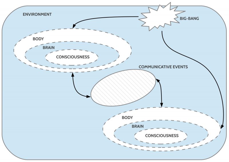
An event space is a space which can be filled up by observable events fitting to the species-specific internal processed environment representations [1], [2] here called internal environments [ENVint]. Thus the same external environment [ENV] can be represented in the presence of  10 different species  in 10 different internal formats. Thus the expression ‘environment’ [ENV] is an abstract concept assuming an objective reality which is common to all living species but indeed it is processed by every species in a species-specific way.

In a human culture the usual point of view [ENVhum] is simultaneous with all the other points of views [ENVa] of all the other other species a.

In the ideal case it would be possible to translate all species-specific views ENVa into a symbolic representation which in turn could then be translated into the human point of view ENVhum. Then — in the ideal case — we could define the term environment [ENV] as the sum of all the different species-specific views translated in a human specific language: ∑ENVa = ENV.

But, because such a generalized view of the environment is until today not really possible by  practical reasons we will use here for the beginning only expressions related to the human specific point of view [ENVhum] using as language an ordinary language [L], here  the English language [LEN]. Every scientific language — e.g. the language of physics — is understood here as a sub language of the ordinary language.

EVENTS

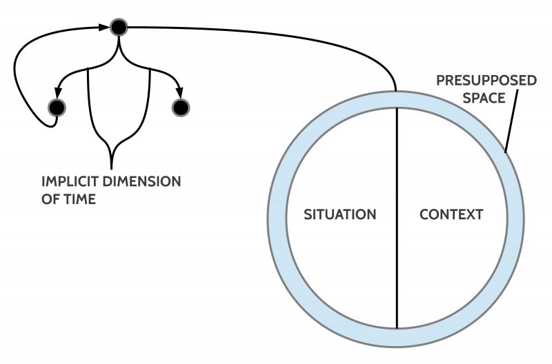
An event [EV] within an event space [ENVa] is a change [X] which can be observed at least from the  members of that species [SP] a which is part of that environment ENV which enables  a species-specific event space [ENVa]. Possibly there can be other actors around in the environment ENV from different species with their specific event space [ENVa] where the content of the different event spaces  can possible   overlap with regard to  certain events.

A behavior is some observable movement of the body of some actor.

Changes X can be associated with certain behavior of certain actors or with non-actor conditions.

Thus when there are some human or non-human  actors in an environment which are moving than they show a behavior which can eventually be associated with some observable changes.
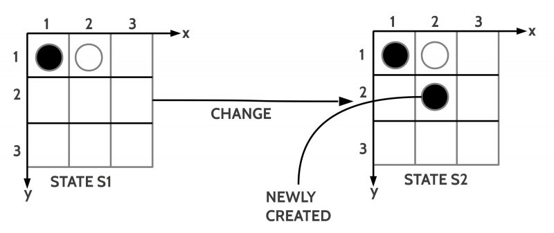
CHANGE

Besides being   associated with observable events in the (species specific) environment the expression  change is understood here as a kind of inner state in an actor which can compare past (stored) states Spast with an actual state SnowIf the past and actual state differ in some observable aspect Diff(Spast, Snow) ≠ 0, then there exists some change X, or Diff(Spast, Snow) = X. Usually the actor perceiving a change X will assume that this internal structure represents something external to the brain, but this must not necessarily be the case. It is of help if there are other human actors which confirm such a change perception although even this does not guarantee that there really is a  change occurring. In the real world it is possible that a whole group of human actors can have a wrong interpretation.

SYMBOLIC COMMUNICATION AND MEANING

It is a specialty of human actors — to some degree shared by other non-human biological actors — that they not only can built up internal representations ENVint of the reality external to the  brain (the body itself or the world beyond the body) which are mostly unconscious, partially conscious, but also they can built up structures of expressions of an internal language Lint which can be mimicked to a high degree by expressions in the body-external environment ENV called expressions of an ordinary language L.

For this to work one  has  to assume that there exists an internal mapping from internal representations ENVint into the expressions of the internal language   Lint as

meaning : ENVint <—> Lint.

and

speaking: Lint —> L

hearing: Lint <— L

Thus human actors can use their ordinary language L to activate internal encodings/ decodings with regard to the internal representations ENVint  gained so far. This is called here symbolic communication.

NO SPEECH ACTS

To classify the occurrences of symbolic expressions during a symbolic communication  is a nearly infinite undertaking. First impressions of the unsolvability of such a classification task can be gained if one reads the Philosophical Investigations of Ludwig Wittgenstein. [5] Later trials from different philosophers and scientists  — e.g. under the heading of speech acts [4] — can  not fully convince until today.

Instead of assuming here a complete scientific framework to classify  occurrences of symbolic expressions of an ordinary language L we will only look to some examples and discuss these.

KINDS OF EXPRESSIONS

In what follows we will look to some selected examples of symbolic expressions and discuss these.

(Decidable) Concrete Expressions [(D)CE]

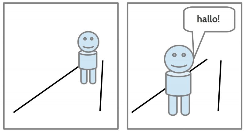
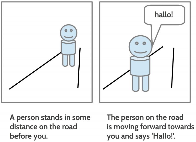
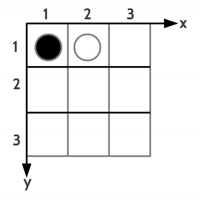
It is assumed here that two human actors A and B  speaking the same ordinary language L  are capable in a concrete situation S to describe objects  OBJ and properties PROP of this situation in a way, that the hearer of a concrete expression E can decide whether the encoded meaning of that expression produced by the speaker is part of the observable situation S or not.

Thus, if A and B are together in a room with a wooden  white table and there is a enough light for an observation then   B can understand what A is saying if he states ‘There is a white wooden table.

To understand means here that both human actors are able to perceive the wooden white table as an object with properties, their brains will transform these external signals into internal neural signals forming an inner — not 1-to-1 — representation ENVint which can further be mapped by the learned meaning function into expressions of the inner language Lint and mapped further — by the speaker — into the external expressions of the learned ordinary language L and if the hearer can hear these spoken expressions he can translate the external expressions into the internal expressions which can be mapped onto the learned internal representations ENVint. In everyday situations there exists a high probability that the hearer then can respond with a spoken ‘Yes, that’s true’.

If this happens that some human actor is uttering a symbolic expression with regard to some observable property of the external environment  and the other human actor does respond with a confirmation then such an utterance is called here a decidable symbolic expression of the ordinary language L. In this case one can classify such an expression  as being true. Otherwise the expression  is classified as being not true.

The case of being not true is not a simple case. Being not true can mean: (i) it is actually simply not given; (ii) it is conceivable that the meaning could become true if the external situation would be  different; (iii) it is — in the light of the accessible knowledge — not conceivable that the meaning could become true in any situation; (iv) the meaning is to fuzzy to decided which case (i) – (iii) fits.

Cognitive Abstraction Processes

Before we talk about (Undecidable) Universal Expressions [(U)UE] it has to clarified that the internal mappings in a human actor are not only non-1-to-1 mappings but they are additionally automatic transformation processes of the kind that concrete perceptions of concrete environmental matters are automatically transformed by the brain into different kinds of states which are abstracted states using the concrete incoming signals as a  trigger either to start a new abstracted state or to modify an existing abstracted state. Given such abstracted states there exist a multitude of other neural processes to process these abstracted states further embedded  in numerous  different relationships.

Thus the assumed internal language Lint does not map the neural processes  which are processing the concrete events as such but the processed abstracted states! Language expressions as such can never be related directly to concrete material because this concrete material  has no direct  neural basis.  What works — completely unconsciously — is that the brain can detect that an actual neural pattern nn has some similarity with a  given abstracted structure NN  and that then this concrete pattern nn  is internally classified as an instance of NN. That means we can recognize that a perceived concrete matter nn is in ‘the light of’ our available (unconscious) knowledge an NN, but we cannot argue explicitly why. The decision has been processed automatically (unconsciously), but we can become aware of the result of this unconscious process.

Universal (Undecidable) Expressions [U(U)E]

Let us repeat the expression ‘There is a white wooden table‘ which has been used before as an example of a concrete decidable expression.

If one looks to the different parts of this expression then the partial expressions ‘white’, ‘wooden’, ‘table’ can be mapped by a learned meaning function φ into abstracted structures which are the result of internal processing. This means there can be countable infinite many concrete instances in the external environment ENV which can be understood as being white. The same holds for the expressions ‘wooden’ and ‘table’. Thus the expressions ‘white’, ‘wooden’, ‘table’ are all related to abstracted structures and therefor they have to be classified as universal expressions which as such are — strictly speaking —  not decidable because they can be true in many concrete situations with different concrete matters. Or take it otherwise: an expression with a meaning function φ pointing to an abstracted structure is asymmetric: one expression can be related to many different perceivable concrete matters but certain members of  a set of different perceived concrete matters can be related to one and the same abstracted structure on account of similarities based on properties embedded in the perceived concrete matter and being part of the abstracted structure.

In a cognitive point of view one can describe these matters such that the expression — like ‘table’ — which is pointing to a cognitive  abstracted structure ‘T’ includes a set of properties Π and every concrete perceived structure ‘t’ (caused e.g. by some concrete matter in our environment which we would classify as a ‘table’) must have a ‘certain amount’ of properties Π* that one can say that the properties  Π* are entailed in the set of properties Π of the abstracted structure T, thus Π* ⊆ Π. In what circumstances some speaker-hearer will say that something perceived concrete ‘is’ a table or ‘is not’ a table will depend from the learning history of this speaker-hearer. A child in the beginning of learning a language L can perhaps call something   a ‘chair’ and the parents will correct the child and will perhaps  say ‘no, this is table’.

Thus the expression ‘There is a white wooden table‘ as such is not true or false because it is not clear which set of concrete perceptions shall be derived from the possible internal meaning mappings, but if a concrete situation S is given with a concrete object with concrete properties then a speaker can ‘translate’ his/ her concrete perceptions with his learned meaning function φ into a composed expression using universal expressions.  In such a situation where the speaker is  part of  the real situation S he/ she  can recognize that the given situation is an  instance of the abstracted structures encoded in the used expression. And recognizing this being an instance interprets the universal expression in a way  that makes the universal expression fitting to a real given situation. And thereby the universal expression is transformed by interpretation with φ into a concrete decidable expression.

SUMMING UP

Thus the decisive moment of turning undecidable universal expressions U(U)E into decidable concrete expressions (D)CE is a human actor A behaving as a speaker-hearer of the used  language L. Without a speaker-hearer every universal expressions is undefined and neither true nor false.

makedecidable :  S x Ahum x E —> E x {true, false}

This reads as follows: If you want to know whether an expression E is concrete and as being concrete is  ‘true’ or ‘false’ then ask  a human actor Ahum which is part of a concrete situation S and the human actor shall  answer whether the expression E can be interpreted such that E can be classified being either ‘true’ or ‘false’.

The function ‘makedecidable()’ is therefore  the description (like a ‘recipe’) of a real process in the real world with real actors. The important factors in this description are the meaning functions inside the participating human actors. Although it is not possible to describe these meaning functions directly one can check their behavior and one can define an abstract model which describes the observable behavior of speaker-hearer of the language L. This is an empirical model and represents the typical case of behavioral models used in psychology, biology, sociology etc.

SOURCES

[1] Jakob Johann Freiherr von Uexküll (German: [ˈʏkskʏl])(1864 – 1944) https://en.wikipedia.org/wiki/Jakob_Johann_von_Uexk%C3%BCll

[2] Jakob von Uexküll, 1909, Umwelt und Innenwelt der Tiere. Berlin: J. Springer. (Download: https://ia802708.us.archive.org/13/items/umweltundinnenwe00uexk/umweltundinnenwe00uexk.pdf )

[3] Wikipedia EN, Speech acts: https://en.wikipedia.org/wiki/Speech_act

[4] Ludwig Josef Johann Wittgenstein ( 1889 – 1951): https://en.wikipedia.org/wiki/Ludwig_Wittgenstein

[5] Ludwig Wittgenstein, 1953: Philosophische Untersuchungen [PU], 1953: Philosophical Investigations [PI], translated by G. E. M. Anscombe /* For more details see: https://en.wikipedia.org/wiki/Philosophical_Investigations */

HMI Analysis for the CM:MI paradigm. Part 3. Actor Story and Theories

Integrating Engineering and the Human Factor (info@uffmm.org)
eJournal uffmm.org ISSN 2567-6458, March 2, 2021,
Author: Gerd Doeben-Henisch
Email: gerd@doeben-henisch.de

Last change: March 2, 2021 13:59h (Minor corrections)

HISTORY

As described in the uffmm eJournal  the wider context of this software project is an integrated  engineering theory called Distributed Actor-Actor Interaction [DAAI] further extended to the Collective Man-Machine Intelligence [CM:MI] paradigm.  This document is part of the Case Studies section.

HMI ANALYSIS, Part 3: Actor Story and  Theories

Context

This text is preceded by the following texts:

Introduction

Having a vision is that moment  where something really new in the whole universe is getting an initial status in some real brain which can enable other neural events which  can possibly be translated in bodily events which finally can change the body-external outside world. If this possibility is turned into reality than the outside world has been changed.

When human persons (groups of homo sapiens specimens) as experts — here acting as stakeholder and intended users as one but in different roles! — have stated a problem and a vision document, then they have to translate these inevitably more fuzzy than clear ideas into the concrete terms of an everyday world, into something which can really work.

To enable a real cooperation  the experts have to generate a symbolic description of their vision (called specification) — using an everyday language, possibly enhanced by special expressions —  in a way that  it can became clear to the whole group, which kind of real events, actions and processes are intended.

In the general case an engineering specification describes concrete forms of entanglements of human persons which enable  these human persons to cooperate   in a real situation. Thereby the translation of  the vision inside the brain  into the everyday body-external reality happens. This is the language of life in the universe.

WRITING A STORY

To elaborate a usable specification can metaphorically be understood  as the writing of a new story: which kinds of actors will do something in certain situations, what kinds of other objects, instruments etc. will be used, what kinds of intrinsic motivations and experiences are pushing individual actors, what are possible outcomes of situations with certain actors, which kind of cooperation is  helpful, and the like. Such a story is  called here  Actor Story [AS].

COULD BE REAL

An Actor Story must be written in a way, that all participating experts can understand the language of the specification in a way that   the content, the meaning of the specification is either decidable real or that it eventually can become real.  At least the starting point of the story should be classifiable as   being decidable actual real. What it means to be decidable actual real has to be defined and agreed between the participating experts before they start writing the Actor Story.

ACTOR STORY [AS]

An Actor Story assumes that the described reality is classifiable as a set of situations (states) and  a situation as part of the Actor Story — abbreviated: situationAS — is understood  as a set of expressions of some everyday language. Every expression being part of an situationAS can be decided as being real (= being true) in the understood real situation.

If the understood real situation is changing (by some event), then the describing situationAS has to be changed too; either some expressions have to be removed or have to be added.

Every kind of change in the real situation S* has to be represented in the actor story with the situationAS S symbolically in the format of a change rule:

X: If condition  C is satisfied in S then with probability π  add to S Eplus and remove from  S Eminus.

or as a formula:

S’π = S + Eplus – Eminus

This reads as follows: If there is an situationAS S and there is a change rule X, then you can apply this change rule X with probability π onto S if the condition of X is satisfied in S. In that case you have to add Eplus to S and you have to remove Eminus from S. The result of these operations is the new (successor) state S’.

The expression C is satisfied in S means, that all elements of C are elements of S too, written as C ⊆ S. The expression add Eplus to S means, that the set Eplus is unified with the set S, written as Eplus ∪ S (or here: Eplus + S). The expression remove Eminus from S means, that the set Eminus is subtracted from the set S, written as S – Eminus.

The concept of apply change rule X to a given state S resulting in S’ is logically a kind of a derivation. Given S,X you will derive by applicating X the new  S’. One can write this as S,X ⊢X S’. The ‘meaning’ of the sign ⊢  is explained above.

Because every successor state S’ can become again a given state S onto which change rules X can be applied — written shortly as X(S)=S’, X(S’)=S”, … — the repeated application of change rules X can generate a whole sequence of states, written as SQ(S,X) = <S’, S”, … Sgoal>.

To realize such a derivation in the real world outside of the thinking of the experts one needs a machine, a computer — formally an automaton — which can read S and X documents and can then can compute the derivation leading to S’. An automaton which is doing such a job is often called a simulator [SIM], abbreviated here as ∑. We could then write with more information:

S,X ⊢ S’

This will read: Given a set S of many states S and a set X of change rules we can derive by an actor story simulator ∑ a successor state S’.

A Model M=<S,X>

In this context of a set S and a set of change rules X we can speak of a model M which is defined by these two sets.

A Theory T=<M,>

Combining a model M with an actor story simulator enables a theory T which allows a set of derivations based on the model, written as SQ(S,X,⊢) = <S’, S”, … Sgoal>. Every derived final state Sgoal in such a derivation is called a theorem of T.

An Empirical Theory Temp

An empirical theory Temp is possible if there exists a theory T with a group of experts which are using this theory and where these experts can interpret the expressions used in theory T by their built-in meaning functions in a way that they always can decide whether the expressions are related to a real situation or not.

Evaluation [ε]

If one generates an Actor Story Theory [TAS] then it can be of practical importance to get some measure how good this theory is. Because measurement is always an operation of comparison between the subject x to be measured and some agreed standard s one has to clarify which kind of a standard for to be good is available. In the general case the only possible source of standards are the experts themselves. In the context of an Actor Story the experts have agreed to some vision [V] which they think to be a better state than a  given state S classified as a problem [P]. These assumptions allow a possible evaluation of a given state S in the ‘light’ of an agreed vision V as follows:

ε: V x S —> |V ⊆ S|[%]
ε(V,S) = |V ⊆ S|[%]

This reads as follows: the evaluation ε is a mapping from the sets V and S into the number of elements from the set V included in the set S converted in the percentage of the number of elements included. Thus if no  element of V is included in the set S then 0% of the vision is realized, if all elements are included then 100%, etc. As more ‘fine grained’ the set V is as more ‘fine grained’  the evaluation can be.

An Evaluated Theory Tε=<M,,ε>

If one combines the concept of a  theory T with the concept of evaluation ε then one can use the evaluation in combination with the derivation in the way that every  state in a derivation SQ(S,X,⊢) = <S’, S”, … Sgoal> will additionally be evaluated, thus one gets sequences of pairs as follows:

SQ(S,X,⊢∑,ε) = <(S’,ε(V,S’)), (S”,ε(V,S”)), …, (Sgoal, ε(V,Sgoal))>

In the ideal case Sgoal is evaluated to 100% ‘good’. In real cases 100% is only an ideal value which usually will only  be approximated until some threshold.

An Evaluated Theory Tε with Algorithmic Intelligence Tε,α=<M,,ε,α>

Because every theory defines a so-called problem space which is here enhanced by some evaluation function one can add an additional operation α (realized by an algorithm) which can repeat the simulator based derivations enhanced with the evaluations to identify those sets of theorems which are qualified as the best theorems according to some criteria given. This operation α is here called algorithmic intelligence of an actor story AS]. The existence of such an algorithmic intelligence of an actor story [αAS] allows the introduction of another derivation concept:

S,X ⊢∑,ε,α S* ⊆  S’

This reads as follows: Given a set S and a set X an evaluated theory with algorithmic intelligence Tε,α can derive a subset S* of all possible theorems S’ where S* matches certain given criteria within V.

WHERE WE ARE NOW

As it should have become clear now the work of HMI analysis is the elaboration of a story which can be done in the format of different kinds of theories all of which can be simulated and evaluated. Even better, the only language you have to know is your everyday language, your mother tongue (mathematics is understood here as a sub-language of the everyday language, which in some special cases can be of some help). For this theory every human person — in all ages! — can be a valuable  colleague to help you in understanding better possible futures. Because all parts of an actor story theory are plain texts, everybody ran read and understand everything. And if different groups of experts have investigated different  aspects of a common field you can merge all texts by only ‘pressing a button’ and you will immediately see how all these texts either work together or show discrepancies. The last effect is a great opportunity  to improve learning and understanding! Together we represent some of the power of life in the universe.

CONTINUATION

See here.


The Simulator as a Learning Artificial Actor [LAA]. Version 1

ISSN 2567-6458, 23.August 2020
Email: info@uffmm.org
Author: Gerd Doeben-Henisch
Email: gerd@doeben-henisch.de

CONTEXT

As described in the uffmm eJournal  the wider context of this software project is a generative theory of cultural anthropology [GCA] which is an extension of the engineering theory called Distributed Actor-Actor Interaction [DAAI]. In  the section Case Studies of the uffmm eJournal there is also a section about Python co-learning – mainly
dealing with python programming – and a section about a web-server with
Dragon. This document will be part of the Case Studies section.

Abstract

The analysis of the main application scenario revealed that classical
logical inference concepts are insufficient for the assistance of human ac-
tors during shared planning. It turned out that the simulator has to be
understood as a real learning artificial actor which has to gain the required
knowledge during the process.

PDF DOCUMENT

LearningArtificialActor-v1 (last change: Aug 23, 2020)

AAI THEORY V2 –A Philosophical Framework

eJournal: uffmm.org,
ISSN 2567-6458, 22.February 2019
Email: info@uffmm.org
Author: Gerd Doeben-Henisch
Email: gerd@doeben-henisch.de

Last change: 23.February 2019 (continued the text)

Last change: 24.February 2019 (extended the text)

CONTEXT

In the overview of the AAI paradigm version 2 you can find this section  dealing with the philosophical perspective of the AAI paradigm. Enjoy reading (or not, then send a comment :-)).

THE DAILY LIFE PERSPECTIVE

The perspective of Philosophy is rooted in the everyday life perspective. With our body we occur in a space with other bodies and objects; different features, properties  are associated with the objects, different kinds of relations an changes from one state to another.

From the empirical sciences we have learned to see more details of the everyday life with regard to detailed structures of matter and biological life, with regard to the long history of the actual world, with regard to many interesting dynamics within the objects, within biological systems, as part of earth, the solar system and much more.

A certain aspect of the empirical view of the world is the fact, that some biological systems called ‘homo sapiens’, which emerged only some 300.000 years ago in Africa, show a special property usually called ‘consciousness’ combined with the ability to ‘communicate by symbolic languages’.

General setting of the homo sapiens species (simplified)
Figure 1: General setting of the homo sapiens species (simplified)

As we know today the consciousness is associated with the brain, which in turn is embedded in the body, which  is further embedded in an environment.

Thus those ‘things’ about which we are ‘conscious’ are not ‘directly’ the objects and events of the surrounding real world but the ‘constructions of the brain’ based on actual external and internal sensor inputs as well as already collected ‘knowledge’. To qualify the ‘conscious things’ as ‘different’ from the assumed ‘real things’ ‘outside there’ it is common to speak of these brain-generated virtual things either as ‘qualia’ or — more often — as ‘phenomena’ which are  different to the assumed possible real things somewhere ‘out there’.

PHILOSOPHY AS FIRST PERSON VIEW

‘Philosophy’ has many facets.  One enters the scene if we are taking the insight into the general virtual character of our primary knowledge to be the primary and irreducible perspective of knowledge.  Every other more special kind of knowledge is necessarily a subspace of this primary phenomenological knowledge.

There is already from the beginning a fundamental distinction possible in the realm of conscious phenomena (PH): there are phenomena which can be ‘generated’ by the consciousness ‘itself’  — mostly called ‘by will’ — and those which are occurring and disappearing without a direct influence of the consciousness, which are in a certain basic sense ‘given’ and ‘independent’,  which are appearing  and disappearing according to ‘their own’. It is common to call these independent phenomena ’empirical phenomena’ which represent a true subset of all phenomena: PH_emp  PH. Attention: These empirical phenomena’ are still ‘phenomena’, virtual entities generated by the brain inside the brain, not directly controllable ‘by will’.

There is a further basic distinction which differentiates the empirical phenomena into those PH_emp_bdy which are controlled by some processes in the body (being tired, being hungry, having pain, …) and those PH_emp_ext which are controlled by objects and events in the environment beyond the body (light, sounds, temperature, surfaces of objects, …). Both subsets of empirical phenomena are different: PH_emp_bdy PH_emp_ext = 0. Because phenomena usually are occurring  associated with typical other phenomena there are ‘clusters’/ ‘pattern’ of phenomena which ‘represent’ possible events or states.

Modern empirical science has ‘refined’ the concept of an empirical phenomenon by introducing  ‘standard objects’ which can be used to ‘compare’ some empirical phenomenon with such an empirical standard object. Thus even when the perception of two different observers possibly differs somehow with regard to a certain empirical phenomenon, the additional comparison with an ’empirical standard object’ which is the ‘same’ for both observers, enhances the quality, improves the precision of the perception of the empirical phenomena.

From these considerations we can derive the following informal definitions:

  1. Something is ‘empirical‘ if it is the ‘real counterpart’ of a phenomenon which can be observed by other persons in my environment too.
  2. Something is ‘standardized empirical‘ if it is empirical and can additionally be associated with a before introduced empirical standard object.
  3. Something is ‘weak empirical‘ if it is the ‘real counterpart’ of a phenomenon which can potentially be observed by other persons in my body as causally correlated with the phenomenon.
  4. Something is ‘cognitive‘ if it is the counterpart of a phenomenon which is not empirical in one of the meanings (1) – (3).

It is a common task within philosophy to analyze the space of the phenomena with regard to its structure as well as to its dynamics.  Until today there exists not yet a complete accepted theory for this subject. This indicates that this seems to be some ‘hard’ task to do.

BRIDGING THE GAP BETWEEN BRAINS

As one can see in figure 1 a brain in a body is completely disconnected from the brain in another body. There is a real, deep ‘gap’ which has to be overcome if the two brains want to ‘coordinate’ their ‘planned actions’.

Luckily the emergence of homo sapiens with the new extended property of ‘consciousness’ was accompanied by another exciting property, the ability to ‘talk’. This ability enabled the creation of symbolic languages which can help two disconnected brains to have some exchange.

But ‘language’ does not consist of sounds or a ‘sequence of sounds’ only; the special power of a language is the further property that sequences of sounds can be associated with ‘something else’ which serves as the ‘meaning’ of these sounds. Thus we can use sounds to ‘talk about’ other things like objects, events, properties etc.

The single brain ‘knows’ about the relationship between some sounds and ‘something else’ because the brain is able to ‘generate relations’ between brain-structures for sounds and brain-structures for something else. These relations are some real connections in the brain. Therefore sounds can be related to ‘something  else’ or certain objects, and events, objects etc.  can become related to certain sounds. But these ‘meaning relations’ can only ‘bridge the gap’ to another brain if both brains are using the same ‘mapping’, the same ‘encoding’. This is only possible if the two brains with their bodies share a real world situation RW_S where the perceptions of the both brains are associated with the same parts of the real world between both bodies. If this is the case the perceptions P(RW_S) can become somehow ‘synchronized’ by the shared part of the real world which in turn is transformed in the brain structures P(RW_S) —> B_S which represent in the brain the stimulating aspects of the real world.  These brain structures B_S can then be associated with some sound structures B_A written as a relation  MEANING(B_S, B_A). Such a relation  realizes an encoding which can be used for communication. Communication is using sound sequences exchanged between brains via the body and the air of an environment as ‘expressions’ which can be recognized as part of a learned encoding which enables the receiving brain to identify a possible meaning candidate.

DIFFERENT MODES TO EXPRESS MEANING

Following the evolution of communication one can distinguish four important modes of expressing meaning, which will be used in this AAI paradigm.

VISUAL ENCODING

A direct way to express the internal meaning structures of a brain is to use a ‘visual code’ which represents by some kinds of drawing the visual shapes of objects in the space, some attributes of  shapes, which are common for all people who can ‘see’. Thus a picture and then a sequence of pictures like a comic or a story board can communicate simple ideas of situations, participating objects, persons and animals, showing changes in the arrangement of the shapes in the space.

Pictorial expressions representing aspects of the visual and the auditory sens modes
Figure 2: Pictorial expressions representing aspects of the visual and the auditory sens modes

Even with a simple visual code one can generate many sequences of situations which all together can ‘tell a story’. The basic elements are a presupposed ‘space’ with possible ‘objects’ in this space with different positions, sizes, relations and properties. One can even enhance these visual shapes with written expressions of  a spoken language. The sequence of the pictures represents additionally some ‘timely order’. ‘Changes’ can be encoded by ‘differences’ between consecutive pictures.

FROM SPOKEN TO WRITTEN LANGUAGE EXPRESSIONS

Later in the evolution of language, much later, the homo sapiens has learned to translate the spoken language L_s in a written format L_w using signs for parts of words or even whole words.  The possible meaning of these written expressions were no longer directly ‘visible’. The meaning was now only available for those people who had learned how these written expressions are associated with intended meanings encoded in the head of all language participants. Thus only hearing or reading a language expression would tell the reader either ‘nothing’ or some ‘possible meanings’ or a ‘definite meaning’.

A written textual version in parallel to a pictorial version
Figure 3: A written textual version in parallel to a pictorial version

If one has only the written expressions then one has to ‘know’ with which ‘meaning in the brain’ the expressions have to be associated. And what is very special with the written expressions compared to the pictorial expressions is the fact that the elements of the pictorial expressions are always very ‘concrete’ visual objects while the written expressions are ‘general’ expressions allowing many different concrete interpretations. Thus the expression ‘person’ can be used to be associated with many thousands different concrete objects; the same holds for the expression ‘road’, ‘moving’, ‘before’ and so on. Thus the written expressions are like ‘manufacturing instructions’ to search for possible meanings and configure these meanings to a ‘reasonable’ complex matter. And because written expressions are in general rather ‘abstract’/ ‘general’ which allow numerous possible concrete realizations they are very ‘economic’ because they use minimal expressions to built many complex meanings. Nevertheless the daily experience with spoken and written expressions shows that they are continuously candidates for false interpretations.

FORMAL MATHEMATICAL WRITTEN EXPRESSIONS

Besides the written expressions of everyday languages one can observe later in the history of written languages the steady development of a specialized version called ‘formal languages’ L_f with many different domains of application. Here I am  focusing   on the formal written languages which are used in mathematics as well as some pictorial elements to ‘visualize’  the intended ‘meaning’ of these formal mathematical expressions.

Properties of an acyclic directed graph with nodes (vertices) and edges (directed edges = arrows)
Fig. 4: Properties of an acyclic directed graph with nodes (vertices) and edges (directed edges = arrows)

One prominent concept in mathematics is the concept of a ‘graph’. In  the basic version there are only some ‘nodes’ (also called vertices) and some ‘edges’ connecting the nodes.  Formally one can represent these edges as ‘pairs of nodes’. If N represents the set of nodes then N x N represents the set of all pairs of these nodes.

In a more specialized version the edges are ‘directed’ (like a ‘one way road’) and also can be ‘looped back’ to a node   occurring ‘earlier’ in the graph. If such back-looping arrows occur a graph is called a ‘cyclic graph’.

Directed cyclic graph extended to represent 'states of affairs'
Fig.5: Directed cyclic graph extended to represent ‘states of affairs’

If one wants to use such a graph to describe some ‘states of affairs’ with their possible ‘changes’ one can ‘interpret’ a ‘node’ as  a state of affairs and an arrow as a change which turns one state of affairs S in a new one S’ which is minimally different to the old one.

As a state of affairs I  understand here a ‘situation’ embedded in some ‘context’ presupposing some common ‘space’. The possible ‘changes’ represented by arrows presuppose some dimension of ‘time’. Thus if a node n’  is following a node n indicated by an arrow then the state of affairs represented by the node n’ is to interpret as following the state of affairs represented in the node n with regard to the presupposed time T ‘later’, or n < n’ with ‘<‘ as a symbol for a timely ordering relation.

Example of a state of affairs with a 2-dimensional space configured as a grid with a black and a white token
Fig.6: Example of a state of affairs with a 2-dimensional space configured as a grid with a black and a white token

The space can be any kind of a space. If one assumes as an example a 2-dimensional space configured as a grid –as shown in figure 6 — with two tokens at certain positions one can introduce a language to describe the ‘facts’ which constitute the state of affairs. In this example one needs ‘names for objects’, ‘properties of objects’ as well as ‘relations between objects’. A possible finite set of facts for situation 1 could be the following:

  1. TOKEN(T1), BLACK(T1), POSITION(T1,1,1)
  2. TOKEN(T2), WHITE(T2), POSITION(T2,2,1)
  3. NEIGHBOR(T1,T2)
  4. CELL(C1), POSITION(1,2), FREE(C1)

‘T1’, ‘T2’, as well as ‘C1’ are names of objects, ‘TOKEN’, ‘BACK’ etc. are names of properties, and ‘NEIGHBOR’ is a relation between objects. This results in the equation:

S1 = {TOKEN(T1), BLACK(T1), POSITION(T1,1,1), TOKEN(T2), WHITE(T2), POSITION(T2,2,1), NEIGHBOR(T1,T2), CELL(C1), POSITION(1,2), FREE(C1)}

These facts describe the situation S1. If it is important to describe possible objects ‘external to the situation’ as important factors which can cause some changes then one can describe these objects as a set of facts  in a separated ‘context’. In this example this could be two players which can move the black and white tokens and thereby causing a change of the situation. What is the situation and what belongs to a context is somewhat arbitrary. If one describes the agriculture of some region one usually would not count the planets and the atmosphere as part of this region but one knows that e.g. the sun can severely influence the situation   in combination with the atmosphere.

Change of a state of affairs given as a state which will be enhanced by a new object
Fig.7: Change of a state of affairs given as a state which will be enhanced by a new object

Let us stay with a state of affairs with only a situation without a context. The state of affairs is     a ‘state’. In the example shown in figure 6 I assume a ‘change’ caused by the insertion of a new black token at position (2,2). Written in the language of facts L_fact we get:

  1. TOKEN(T3), BLACK(T3), POSITION(2,2), NEIGHBOR(T3,T2)

Thus the new state S2 is generated out of the old state S1 by unifying S1 with the set of new facts: S2 = S1 {TOKEN(T3), BLACK(T3), POSITION(2,2), NEIGHBOR(T3,T2)}. All the other facts of S1 are still ‘valid’. In a more general manner one can introduce a change-expression with the following format:

<S1, S2, add(S1,{TOKEN(T3), BLACK(T3), POSITION(2,2), NEIGHBOR(T3,T2)})>

This can be read as follows: The follow-up state S2 is generated out of the state S1 by adding to the state S1 the set of facts { … }.

This layout of a change expression can also be used if some facts have to be modified or removed from a state. If for instance  by some reason the white token should be removed from the situation one could write:

<S1, S2, subtract(S1,{TOKEN(T2), WHITE(T2), POSITION(2,1)})>

Another notation for this is S2 = S1 – {TOKEN(T2), WHITE(T2), POSITION(2,1)}.

The resulting state S2 would then look like:

S2 = {TOKEN(T1), BLACK(T1), POSITION(T1,1,1), CELL(C1), POSITION(1,2), FREE(C1)}

And a combination of subtraction of facts and addition of facts would read as follows:

<S1, S2, subtract(S1,{TOKEN(T2), WHITE(T2), POSITION(2,1)}, add(S1,{TOKEN(T3), BLACK(T3), POSITION(2,2)})>

This would result in the final state S2:

S2 = {TOKEN(T1), BLACK(T1), POSITION(T1,1,1), CELL(C1), POSITION(1,2), FREE(C1),TOKEN(T3), BLACK(T3), POSITION(2,2)}

These simple examples demonstrate another fact: while facts about objects and their properties are independent from each other do relational facts depend from the state of their object facts. The relation of neighborhood e.g. depends from the participating neighbors. If — as in the example above — the object token T2 disappears then the relation ‘NEIGHBOR(T1,T2)’ no longer holds. This points to a hierarchy of dependencies with the ‘basic facts’ at the ‘root’ of a situation and all the other facts ‘above’ basic facts or ‘higher’ depending from the basic facts. Thus ‘higher order’ facts should be added only for the actual state and have to be ‘re-computed’ for every follow-up state anew.

If one would specify a context for state S1 saying that there are two players and one allows for each player actions like ‘move’, ‘insert’ or ‘delete’ then one could make the change from state S1 to state S2 more precise. Assuming the following facts for the context:

  1. PLAYER(PB1), PLAYER(PW1), HAS-THE-TURN(PB1)

In that case one could enhance the change statement in the following way:

<S1, S2, PB1,insert(TOKEN(T3,2,2)),add(S1,{TOKEN(T3), BLACK(T3), POSITION(2,2)})>

This would read as follows: given state S1 the player PB1 inserts a  black token at position (2,2); this yields a new state S2.

With or without a specified context but with regard to a set of possible change statements it can be — which is the usual case — that there is more than one option what can be changed. Some of the main types of changes are the following ones:

  1. RANDOM
  2. NOT RANDOM, which can be specified as follows:
    1. With PROBABILITIES (classical, quantum probability, …)
    2. DETERMINISTIC

Furthermore, if the causing object is an actor which can adapt structurally or even learn locally then this actor can appear in some time period like a deterministic system, in different collected time periods as an ‘oscillating system’ with different behavior, or even as a random system with changing probabilities. This make the forecast of systems with adaptive and/ or learning systems rather difficult.

Another aspect results from the fact that there can be states either with one actor which can cause more than one action in parallel or a state with multiple actors which can act simultaneously. In both cases the resulting total change has eventually to be ‘filtered’ through some additional rules telling what  is ‘possible’ in a state and what not. Thus if in the example of figure 6 both player want to insert a token at position (2,2) simultaneously then either  the rules of the game would forbid such a simultaneous action or — like in a computer game — simultaneous actions are allowed but the ‘geometry of a 2-dimensional space’ would not allow that two different tokens are at the same position.

Another aspect of change is the dimension of time. If the time dimension is not explicitly specified then a change from some state S_i to a state S_j does only mark the follow up state S_j as later. There is no specific ‘metric’ of time. If instead a certain ‘clock’ is specified then all changes have to be aligned with this ‘overall clock’. Then one can specify at what ‘point of time t’ the change will begin and at what point of time t*’ the change will be ended. If there is more than one change specified then these different changes can have different timings.

THIRD PERSON VIEW

Up until now the point of view describing a state and the possible changes of states is done in the so-called 3rd-person view: what can a person perceive if it is part of a situation and is looking into the situation.  It is explicitly assumed that such a person can perceive only the ‘surface’ of objects, including all kinds of actors. Thus if a driver of a car stears his car in a certain direction than the ‘observing person’ can see what happens, but can not ‘look into’ the driver ‘why’ he is steering in this way or ‘what he is planning next’.

A 3rd-person view is assumed to be the ‘normal mode of observation’ and it is the normal mode of empirical science.

Nevertheless there are situations where one wants to ‘understand’ a bit more ‘what is going on in a system’. Thus a biologist can be  interested to understand what mechanisms ‘inside a plant’ are responsible for the growth of a plant or for some kinds of plant-disfunctions. There are similar cases for to understand the behavior of animals and men. For instance it is an interesting question what kinds of ‘processes’ are in an animal available to ‘navigate’ in the environment across distances. Even if the biologist can look ‘into the body’, even ‘into the brain’, the cells as such do not tell a sufficient story. One has to understand the ‘functions’ which are enabled by the billions of cells, these functions are complex relations associated with certain ‘structures’ and certain ‘signals’. For this it is necessary to construct an explicit formal (mathematical) model/ theory representing all the necessary signals and relations which can be used to ‘explain’ the obsrvable behavior and which ‘explains’ the behavior of the billions of cells enabling such a behavior.

In a simpler, ‘relaxed’ kind of modeling  one would not take into account the properties and behavior of the ‘real cells’ but one would limit the scope to build a formal model which suffices to explain the oservable behavior.

This kind of approach to set up models of possible ‘internal’ (as such hidden) processes of an actor can extend the 3rd-person view substantially. These models are called in this text ‘actor models (AM)’.

HIDDEN WORLD PROCESSES

In this text all reported 3rd-person observations are called ‘actor story’, independent whether they are done in a pictorial or a textual mode.

As has been pointed out such actor stories are somewhat ‘limited’ in what they can describe.

It is possible to extend such an actor story (AS)  by several actor models (AM).

An actor story defines the situations in which an actor can occur. This  includes all kinds of stimuli which can trigger the possible senses of the actor as well as all kinds of actions an actor can apply to a situation.

The actor model of such an actor has to enable the actor to handle all these assumed stimuli as well as all these actions in the expected way.

While the actor story can be checked whether it is describing a process in an empirical ‘sound’ way,  the actor models are either ‘purely theoretical’ but ‘behavioral sound’ or they are also empirically sound with regard to the body of a biological or a technological system.

A serious challenge is the occurrence of adaptiv or/ and locally learning systems. While the actor story is a finite  description of possible states and changes, adaptiv or/ and locally learning systeme can change their behavior while ‘living’ in the actor story. These changes in the behavior can not completely be ‘foreseen’!

COGNITIVE EXPERT PROCESSES

According to the preceding considerations a homo sapiens as a biological system has besides many properties at least a consciousness and the ability to talk and by this to communicate with symbolic languages.

Looking to basic modes of an actor story (AS) one can infer some basic concepts inherently present in the communication.

Without having an explicit model of the internal processes in a homo sapiens system one can infer some basic properties from the communicative acts:

  1. Speaker and hearer presuppose a space within which objects with properties can occur.
  2. Changes can happen which presuppose some timely ordering.
  3. There is a disctinction between concrete things and abstract concepts which correspond to many concrete things.
  4. There is an implicit hierarchy of concepts starting with concrete objects at the ‘root level’ given as occurence in a concrete situation. Other concepts of ‘higher levels’ refer to concepts of lower levels.
  5. There are different kinds of relations between objects on different conceptual levels.
  6. The usage of language expressions presupposes structures which can be associated with the expressions as their ‘meanings’. The mapping between expressions and their meaning has to be learned by each actor separately, but in cooperation with all the other actors, with which the actor wants to share his meanings.
  7. It is assume that all the processes which enable the generation of concepts, concept hierarchies, relations, meaning relations etc. are unconscious! In the consciousness one can  use parts of the unconscious structures and processes under strictly limited conditions.
  8. To ‘learn’ dedicated matters and to be ‘critical’ about the quality of what one is learnig requires some disciplin, some learning methods, and a ‘learning-friendly’ environment. There is no guaranteed method of success.
  9. There are lots of unconscious processes which can influence understanding, learning, planning, decisions etc. and which until today are not yet sufficiently cleared up.


BACKGROUND INFORMATION 27.Dec.2018: The AAI-paradigm and Quantum Logic. The Limits of Classic Probability

eJournal: uffmm.org, ISSN 2567-6458
Email: info@uffmm.org
Author: Gerd Doeben-Henisch
Email: gerd@doeben-henisch.de

Last Corrections: 30.Dec.2018

CONTEXT

This is a continuation from the post about QL Basics Concepts Part 1. The general topic here is the analysis of properties of human behavior, actually narrowed down to the statistical properties. From the different possible theories applicable to statistical properties of behavior here the one called CPT (classical probability theory) is selected for a short examination.

SUMMARY

An analysis of the classical probability theory shows that the empirical application of this theory is limited to static sets of events and probabilities. In the case of biological systems which are adaptive with regard to structure and cognition this does not work. This yields the question whether a quantum probability theory approach does work or not.

THE CPT IDEA

  1. Before we are looking  to the case of quantum probability theory (QLPT) let us examine the case of a classical probability theory (CPT) a little bit more.
  2. Generally one has to distinguish the symbolic formal representation of a theory T and some domain of application D distinct from the symbolic representation.
  3. In principle the domain of application D can be nearly anything, very often again another symbolic representation. But in the case of empirical applications we assume usually some subset of ’empirical events’ E of the ’empirical (real) world’ W.
  4. For the following let us assume (for a while) that this is the case, that D is a subset of the empirical world W.
  5. Talking about ‘events in an empirical real world’ presupposes that there there exists a ‘procedure of measurement‘ using a ‘previously defined standard object‘ and a ‘symbolic representation of the measurement results‘.
  6. Furthermore one has to assume a community of ‘observers‘ which have minimal capabilities to ‘observe’, which implies ‘distinctions between different results’, some ‘ordering of successions (before – after)’, to ‘attach symbols according to some rules’ to measurement results, to ‘translate measurement results’ into more abstract concepts and relations.
  7. Thus to speak about empirical results assumes a set of symbolic representations of those events as a finite set of symbolic representations which represent a ‘state in the real world’ which can have a ‘predecessor state before’ and – possibly — a ‘successor state after’ the ‘actual’ state. The ‘quality’ of these measurement representations depends from the quality of the measurement procedure as well as from the quality of the cognitive capabilities of the participating observers.
  8. In the classical probability theory T_cpt as described by Kolmogorov (1932) it is assumed that there is a set E of ‘elementary events’. The set E is assumed to be ‘complete’ with regard to all possible events. The probability P is coming into play with a mapping from E into the set of positive real numbers R+ written as P: E —> R+ or P(E) = 1 with the assumption that all the individual elements e_i of E have an individual probability P(e_i) which obey the rule P(e_1) + P(e_2) + … + P(e_n) = 1.
  9. In the formal theory T_cpt it is not explained ‘how’ the probabilities are realized in the concrete case. In the ‘real world’ we have to identify some ‘generators of events’ G, otherwise we do not know whether an event e belongs to a ‘set of probability events’.
  10. Kolmogorov (1932) speaks about a necessary generator as a ‘set of conditions’ which ‘allows of any number of repetitions’, and ‘a set of events can take place as a result of the establishment of the condition’. (cf. p.3) And he mentions explicitly the case that different variants of the a priori assumed possible events can take place as a set A. And then he speaks of this set A also of an event which has taken place! (cf. p.4)
  11. If one looks to the case of the ‘set A’ then one has to clarify that this ‘set A’ is not an ordinary set of set theory, because in a set every member occurs only once. Instead ‘A’ represents a ‘sequence of events out of the basic set E’. A sequence is in set theory an ‘ordered set’, where some set (e.g. E) is mapped into an initial segment  of the natural numbers Nat and in this case  the set A contains ‘pairs from E x Nat|\n’  with a restriction of the set Nat to some n. The ‘range’ of the set A has then ‘distinguished elements’ whereby the ‘domain’ can have ‘same elements’. Kolmogorov addresses this problem with the remark, that the set A can be ‘defined in any way’. (cf. p.4) Thus to assume the set A as a set of pairs from the Cartesian product E x Nat|\n with the natural numbers taken from the initial segment of the natural numbers is compatible with the remark of Kolmogorov and the empirical situation.
  12. For a possible observer it follows that he must be able to distinguish different states <s1, s2, …, sm> following each other in the real world, and in every state there is an event e_i from the set of a priori possible events E. The observer can ‘count’ the occurrences of a certain event e_i and thus will get after n repetitions for every event e_i a number of occurrences m_i with m_i/n giving the measured empirical probability of the event e_i.
  13. Example 1: Tossing a coin with ‘head (H)’ or ‘tail (T)’ we have theoretically the probabilities ‘1/2’ for each event. A possible outcome could be (with ‘H’ := 0, ‘T’ := 1): <((0,1), (0,2), (0,3), (1,4), (0,5)> . Thus we have m_H = 4, m_T = 1, giving us m_H/n = 4/5 and m_T/n = 1/5. The sum yields m_H/n + m_T/n = 1, but as one can see the individual empirical probabilities are not in accordance with the theory requiring 1/2 for each. Kolmogorov remarks in his text  that if the number of repetitions n is large enough then will the values of the empirically measured probability approach the theoretically defined values. In a simple experiment with a random number generator simulating the tossing of the coin I got the numbers m_Head = 4978, m_Tail = 5022, which gives the empirical probabilities m_Head/1000 = 0.4977 and m_Teil/ 1000 = 0.5021.
  14. This example demonstrates while the theoretical term ‘probability’ is a simple number, the empirical counterpart of the theoretical term is either a simple occurrence of a certain event without any meaning as such or an empirically observed sequence of events which can reveal by counting and division a property which can be used as empirical probability of this event generated by a ‘set of conditions’ which allow the observed number of repetitions. Thus we have (i) a ‘generator‘ enabling the events out of E, we have (ii) a ‘measurement‘ giving us a measurement result as part of an observation, (iii) the symbolic encoding of the measurement result, (iv) the ‘counting‘ of the symbolic encoding as ‘occurrence‘ and (v) the counting of the overall repetitions, and (vi) a ‘mathematical division operation‘ to get the empirical probability.
  15. Example 1 demonstrates the case of having one generator (‘tossing a coin’). We know from other examples where people using two or more coins ‘at the same time’! In this case the set of a priori possible events E is occurring ‘n-times in parallel’: E x … x E = E^n. While for every coin only one of the many possible basic events can occur in one state, there can be n-many such events in parallel, giving an assembly of n-many events each out of E. If we keeping the values of E = {‘H’, ‘T’} then we have four different basic configurations each with probability 1/4. If we define more ‘abstract’ events like ‘both the same’ (like ‘0,0’, ‘1,1’) or ‘both different’ (like ‘0,1’. ‘1,0’), then we have new types of complex events with different probabilities, each 1/2. Thus the case of n-many generators in parallel allows new types of complex events.
  16. Following this line of thinking one could consider cases like (E^n)^n or even with repeated applications of the Cartesian product operation. Thus, in the case of (E^n)^n, one can think of different gamblers each having n-many dices in a cup and tossing these n-many dices simultaneously.
  17. Thus we have something like the following structure for an empirical theory of classical probability: CPT(T) iff T=<G,E,X,n,S,P*>, with ‘G’ as the set of generators producing out of E events according to the layout of the set X in a static (deterministic) manner. Here the  set E is the set of basic events. The set X is a ‘typified set’ constructed out of the set E with t-many applications of the Cartesian operation starting with E, then E^n1, then (E^n1)^n2, …. . ‘n’ denotes the number of repetitions, which determines the length of a sequence ‘S’. ‘P*’ represents the ’empirical probability’ which approaches the theoretical probability P while n is becoming ‘big’. P* is realized as a tuple of tuples according to the layout of the set X  where each element in the range of a tuple  represents the ‘number of occurrences’ of a certain event out of X.
  18. Example: If there is a set E = {0,1} with the layout X=(E^2)^2 then we have two groups with two generators each: <<G1, G2>,<G3,G4>>. Every generator G_i produces events out of E. In one state i this could look like  <<0, 0>,<1,0>>. As part of a sequence S this would look like S = <….,(<<0, 0>,<1,0>>,i), … > telling that in the i-th state of S there is an occurrence of events like shown. The empirical probability function P* has a corresponding layout P* = <<m1, m2>,<m3,m4>> with the m_j as ‘counter’ which are counting the occurrences of the different types of events as m_j =<c_e1, …, c_er>. In the example there are two different types of events occurring {0,1} which requires two counters c_0 and c_1, thus we would have m_j =<c_0, c_1>, which would induce for this example the global counter structure:  P* = <<<c_0, c_1>, <c_0, c_1>>,<<c_0,  c_1>,<c_0, c_1>>>. If the generators are all the same then the set of basic events E is the same and in theory   the theoretical probability function P: E —> R+ would induce the same global values for all generators. But in the empirical case, if the theoretical probability function P is not known, then one has to count and below the ‘magic big n’ the values of the counter of the empirical probability function can be different.
  19. This format of the empirical classical  probability theory CPT can handle the case of ‘different generators‘ which produce events out of the same basic set E but with different probabilities, which can be counted by the empirical probability function P*. A prominent case of different probabilities with the same set of events is the case of manipulations of generators (a coin, a dice, a roulette wheel, …) to deceive other people.
  20. In the examples mentioned so far the probabilities of the basic events as well as the complex events can be different in different generators, but are nevertheless  ‘static’, not changing. Looking to generators like ‘tossing a coin’, ‘tossing a dice’ this seams to be sound. But what if we look to other types of generators like ‘biological systems’ which have to ‘decide’ which possible options of acting they ‘choose’? If the set of possible actions A is static, then the probability of selecting one action a out of A will usually depend from some ‘inner states’ IS of the biological system. These inner states IS need at least the following two components:(i) an internal ‘representation of the possible actions’ IS_A as well (ii) a finite set of ‘preferences’ IS_Pref. Depending from the preferences the biological system will select an action IS_a out of IS_A and then it can generate an action a out of A.
  21. If biological systems as generators have a ‘static’ (‘deterministic’) set of preferences IS_Pref, then they will act like fixed generators for ‘tossing a coin’, ‘tossing a dice’. In this case nothing will change.  But, as we know from the empirical world, biological systems are in general ‘adaptive’ systems which enables two kinds of adaptation: (i) ‘structural‘ adaptation like in biological evolution and (ii) ‘cognitive‘ adaptation as with higher organisms having a neural system with a brain. In these systems (example: homo sapiens) the set of preferences IS_Pref can change in time as well as the internal ‘representation of the possible actions’ IS_A. These changes cause a shift in the probabilities of the events manifested in the realized actions!
  22. If we allow possible changes in the terms ‘G’ and ‘E’ to ‘G+’ and ‘E+’ then we have no longer a ‘classical’ probability theory CPT. This new type of probability theory we can call ‘non-classic’ probability theory NCPT. A short notation could be: NCPT(T) iff T=<G+,E+,X,n,S,P*> where ‘G+’ represents an adaptive biological system with changing representations for possible Actions A* as well as changing preferences IS_Pref+. The interesting question is, whether a quantum logic approach QLPT is a possible realization of such a non-classical probability theory. While it is known that the QLPT works for physical matters, it is an open question whether it works for biological systems too.
  23. REMARK: switching from static generators to adaptive generators induces the need for the inclusion of the environment of the adaptive generators. ‘Adaptation’ is generally a capacity to deal better with non-static environments.

See continuation here.