eJournal: uffmm.org ISSN 2567-6458
27.March 2022 – 27.March 2022
Email: info@uffmm.org
Author: Gerd Doeben-Henisch
Email: gerd@doeben-henisch.de
BLOG-CONTEXT
This post is part of the Oksimo Application theme which is part of the uffmm blog.
PREFACE
This post shows a simple simulation example with the beta-version of the new Version 2 of the oksimo programming environment. This example shall illustrate the concept of an ‘Everyday Empirical Theory‘ as described in this blog 11 days before. It is intentionally as ‘simple as possible’. Probably some more examples will be shown.
FROM THEORY TO AN APPLICATION
To apply a theory concept in an everyday world there are many formats possible. In this text it will be shown how such an application would look like if one is applying the oksimo programming environment. Until now there exists only a German Blog (oksimo.org) describing the oksimo paradigm a little bit. But the examples there are written with oksimo version 1, which didn’t allow to use math. In version 2 this is possible, accompanied by some visual graph features.
Everyday Experts – Basic Ideas

SOME MORE FEATURES
The basic schema of the oksimo paradigm assumes the following components:
- The description of a ‘given situation’ as a ‘start state’.
- The description of a ‘vision’ functioning as a ‘goal’ which allows a basic ‘Benchmarking’.
- A list of ‘change rules’ which describe the assumed possible changes
- An ‘inference engine’ called ‘simulator’: Depending from the number of wanted ‘simulation cycles’ (‘inferences’) the simulator applies the change rules onto a given state S and thereby it is producing a ‘follow up state’ S*, which becomes the new given state. The series of generated states represents the ‘history’ of a simulation. Every follow up state is an ‘inference’ and by definition also a ‘forecast’.
All these features (1) – (4) together constitute a full empirical theory in the sense of the mentioned theory post before.
Let us look to a real simulation.
A REAL SIMULATION
The following example has been run with Oksimo v2.0 (Pre-Release) (353e5). Hopefully we can finish the pre-release to a full release the next few weeks.
A VISION
Name: v2026
Expressions:
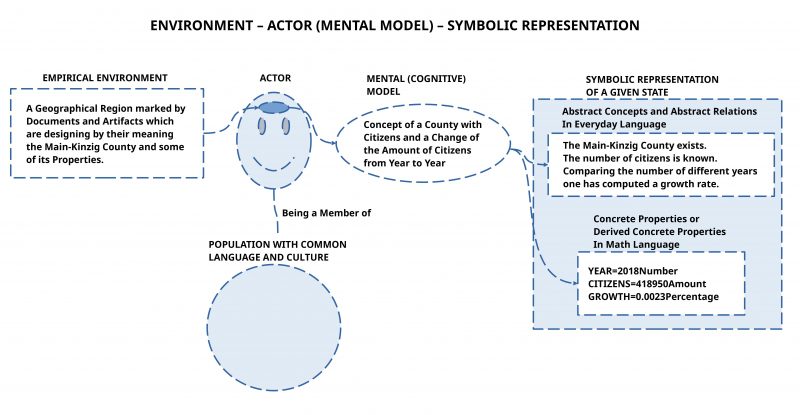
The Main-Kinzig County exists.
Math expressions:
YEAR>2025 and YEAR<2027
This simple goal assumes the existence of the Main-Kinzig County for the year 2026.
GIVEN START STATE
Name: StartSimple1
Expressions:
The Main-Kinzig County exists.
The number of citizens is known.
Comparing the number of different years one has computed a growth rate.
Math expressions:
YEAR=2018Number
CITIZENS=418950Amount
GROWTH=0.0023Percentage
The start state makes some simple statements which are assumed to be ‘valid’ in a ‘real given situation’ by the participating natural experts.
CHANGE RULES
In this example there is only one change rules (In principle there can be as many change rules as wanted).
Rule name: Growth1
Probability: 1.0
Conditions:
The Main-Kinzig County exists.
Math conditions:
CITIZENS < 450000
Effects plus:
Effects minus:
Effects math:
CITIZENS=CITIZENS+(CITIZENS*GROWTH)
YEAR=YEAR+1
This change rules is rather simple. It looks only to the fact whether the Main-Kinzig County exists and wether the number of citizens is still below 450000. If this is the case, then the year will be incremented and the number of citizens will be incremented according to an extremely simple formula.
For every named quantity in this simulation (YEAR, GROWTH, CITIZENS) the values are collected for every simulation cycle and therefore can be used for evaluations. In this simple case only the quantities of YEAR and CITIZENS have changes:
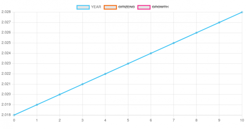

Here the quick log of simulation cycle round 7 – 9:
Round 7

State rules:
Vision rules:
Current states: The number of citizens is known.,Comparing the number of different years one has computed a growth rate.,The Main-Kinzig County exists.
Current visions: The Main-Kinzig County exists.
Current values:
YEAR: 2025Number
CITIZENS: 425741.8149741673Amount
GROWTH: 0.0023Percentage

50.00 percent of your vision was achieved by reaching the following states:
The Main-Kinzig County exists.,
And the following math visions:
None

Round 8

State rules:
Vision rules:
Current states: The number of citizens is known.,Comparing the number of different years one has computed a growth rate.,The Main-Kinzig County exists.
Current visions: The Main-Kinzig County exists.
Current values:
YEAR: 2026Number
CITIZENS: 426721.0211486079Amount
GROWTH: 0.0023Percentage

100.00 percent of your vision was achieved by reaching the following states:
The Main-Kinzig County exists.,
And the following math visions:
YEAR>2025 and YEAR<2027,

Round 9

State rules:
Vision rules:
Current states: The number of citizens is known.,Comparing the number of different years one has computed a growth rate.,The Main-Kinzig County exists.
Current visions: The Main-Kinzig County exists.
Current values:
YEAR: 2027Number
CITIZENS: 427702.4794972497Amount
GROWTH: 0.0023Percentage

50.00 percent of your vision was achieved by reaching the following states:
The Main-Kinzig County exists.,
And the following math visions:
None
In round 8 one can see, that the simulation announces:
“100.00 percent of your vision was achieved by reaching the following states: The Main-Kinzig County exists., And the following math visions: YEAR>2025 and YEAR<2027“
From this the natural expert can conclude that his requirements given in the vision are ‘fulfilled’/’satisfied’.
WHAT COMES NEXT?
In a loosely order more examples will follow. Here you find the next one.
