eJournal: uffmm.org ISSN 2567-6458
30.March 2022 – 31.March 2022, 11:55h
Email: info@uffmm.org
Author: Gerd Doeben-Henisch
Email: gerd@doeben-henisch.de
BLOG-CONTEXT
This post is part of the Oksimo Application theme which is part of the uffmm blog.
PREFACE
This post shows a continuation from the simple simulation example in the preceding post. It points to an implicit problem of the demographic modeling of the Main-Kinzig County (German: Main-Kinzig Kreis [MKK]) only using the official numbers available in the World Wide Web from the Hessian statistical office. Some questions arise without giving an answer in this post.
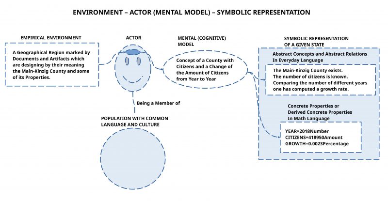
A REAL SIMULATION
The following example has been run with Oksimo v2.0 (Pre-Release) (c972). Hopefully we can finish the pre-release to a full release the next few days.
STRUCTURE OF THE SIMULATION
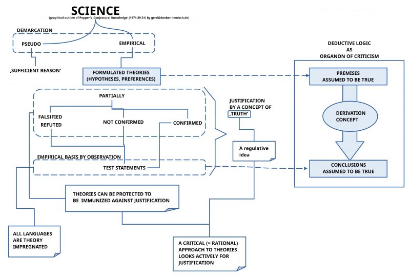
The structure of the simulation follows the schema of an empirical theory as follows:
- A ‘given situation’ will be described which is assumed to be ’empirically sound’ by the authors.
- A ‘state in the future’ (‘vision’, ‘goal’ ‘forecast’) is given for benchmarking.
- At least one ‘change rule’ is given representing an ‘inference rule’ for everyday experience.
- The ‘inference engine’ for making a ‘logical deduction’ is ‘hidden’ in the ‘simulator’, which is doing the job of applying the change rules to a given situation.
Here the concrete definitions:
VISION
Name: vmkkdemo1
Expressions:
The Main-Kinzig County exists.
Math expressions:
YEAR>2032
GIVEN STATE
Name: smkkDemo1
Expressions:
The Main-Kinzig County exists.
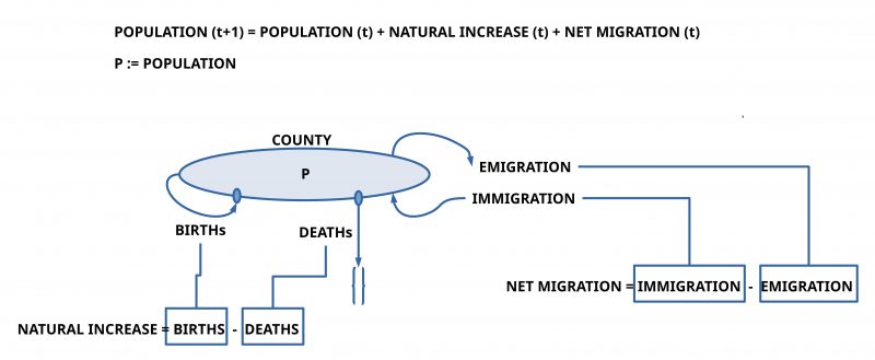
The number of citizens is known.
Based on preceding years a growth rate could be computed.
A growth rate has two components: natural increase and net migration.
The component natural increase has again two components: the rates of births and deaths.
The net migration is based on rates for immigration and emigrations.
The number for a population in a year t+1 is the product of the population of the preceding year t enriched with the natural increase and the net migration.
Math expressions:
IMMIGRATION=18000Amount
EMIGRATION=15900Amount
NETMIGR=0Number
BIRTHS=59400Amount
DEATHS=70000Amount
NATINCREASE=0Number
CITIZENS=421689Amount
YEAR=2020Number
CHANGE RULE (Inference Rule)
(Attention: There can be arbitrary many rules; here only one is used)
Rule name: rworld1
Probability: 1.0
Conditions:
The Main-Kinzig County exists.
Math conditions:
YEAR>=0
Effects plus:
Effects minus:
Effects math:
YEAR=YEAR+1
NETMIGR=IMMIGRATION-EMIGRATION
NATINCREASE=BIRTHS-DEATHS
CITIZENS=CITIZENS+NATINCREASE+NETMIGR
SIMULATION
simmkkDemo2
Selected visions:
vmkkdemo1
Selected states:
smkkDemo1
Selected rules:
rworld1
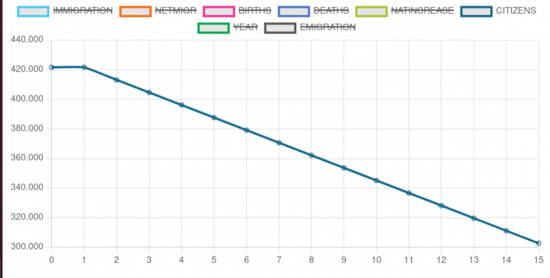
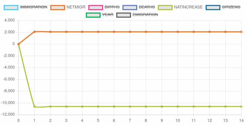
GRAPH CITIZENS
GRAPH NETMIGR NATINCREASE
Here the log protocol from simulation cycles 12-13:
Round 12

State rules:
rworld1 applied  (Prob: 100 Rand: 11/100)
Math applied:
CITIZENS=CITIZENS+NATINCREASE+NETMIGR
NATINCREASE=BIRTHS-DEATHS
YEAR=YEAR+1
NETMIGR=IMMIGRATION-EMIGRATION
Vision rules:
Current states: The number of citizens is known.,The component natural increase has again two components: the rates of births and deaths.,The net migration is based on rates for immigration and emigrations.,The Main-Kinzig County exists.,A growth rate has two components: natural increase and net migration.,The number for a population in a year t+1 is the product of the population of the preceding year t enriched with the natural increase and the net migration.,Based on preceding years a growth rate could be computed.
Current visions: The Main-Kinzig County exists.
Current values:
IMMIGRATION: 18000Amount
NETMIGR: 2100Number
BIRTHS: 59400Amount
DEATHS: 70000Amount
NATINCREASE: -10600Number
CITIZENS: 328189Amount
YEAR: 2032Number
EMIGRATION: 15900Amount

50.00 percent of your vision was achieved by reaching the following states:
The Main-Kinzig County exists.,
And the following math visions:
None

Round 13

State rules:
rworld1 applied  (Prob: 100 Rand: 63/100)
Math applied:
CITIZENS=CITIZENS+NATINCREASE+NETMIGR
NATINCREASE=BIRTHS-DEATHS
YEAR=YEAR+1
NETMIGR=IMMIGRATION-EMIGRATION
Vision rules:
Current states: The number of citizens is known.,The component natural increase has again two com
ponents: the rates of births and deaths.,The net migration is based on rates for immigration and
emigrations.,The Main-Kinzig County exists.,A growth rate has two components: natural increase an
d net migration.,The number for a population in a year t+1 is the product of the population of th
e preceding year t enriched with the natural increase and the net migration.,Based on preceding y
ears a growth rate could be computed.
Current visions: The Main-Kinzig County exists.
Current values:
IMMIGRATION: 18000Amount
NETMIGR: 2100Number
BIRTHS: 59400Amount
DEATHS: 70000Amount
NATINCREASE: -10600Number
CITIZENS: 319689Amount
YEAR: 2033Number
EMIGRATION: 15900Amount

100.00 percent of your vision was achieved by reaching the following states:
The Main-Kinzig County exists.,
And the following math visions:
YEAR>2032
One can see here that the simulator announces a 100% satisfaction of the goal because the year 2032 has been passed and the Main-Kinzig County still exists.
DISCUSSION
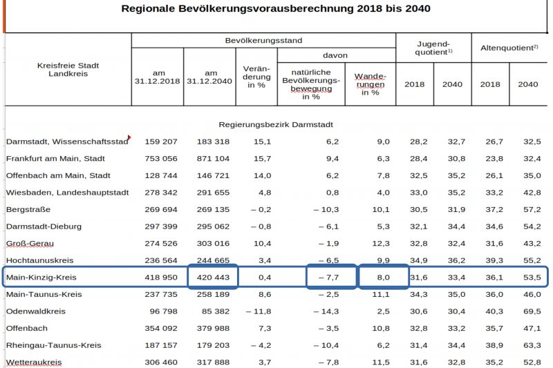
Although the shown simulation is still extremely simple it points to a hidden problem of the official demographic data. The hessian statistical office computes a forecast for the MKK in 2040 with 420443 citizens starting with the year 2018. [3] Comparing these numbers with those from the demographic changes between 1.January 2021 and 30.June 2021 [2] then one gets a real difference: NATINCREASE -7.7 becomes -0.15% and NETMIGR 8.0 becomes 0.21%. This results in a 6-month fraction of about -736 to -635 for NATINCREASE and of about 764 to 889 for NETMIGR.
These observations point (i) to the general problem of getting ‘good data’ and (ii) at the same time how fragile the data are. With rather constant rates in births and deaths the migration data can change a lot. For 2020-2021 we have with 2.107 a NETMIGR rate of about 0.5%. [1] What now are the ‘real data’?
A DIFFERENT SIMULATION
Until now we have only data from single points of time (2018, 2021 (2040)) or of a small time window (1.January 2021, 30.June 2021). If we would take the data from the time window (Jan 2021, Jun 2021) and if we take the change rates from these data as percentage of the final value of citizens, then we are producing another graph knowing, that this clearly will not represent ‘the empirical reality’ sufficiently well. Nevertheless it can help to get some ‘awareness’ that the real numbers deserve more research, especially related to their ‘dynamics’ which is embedded in rather complex clusters of different factors interacting with each other.[4]
STRUCTURE OF SIMULATION
GIVEN SITUATION
TEXT
Name: smkkDemo2
The Main-Kinzig County exists.
The number of citizens is known.
Based on preceding years a growth rate could be computed.
A growth rate has two components: natural increase and net migration.
The component natural increase has again two components: the rates of births and deaths.
The net migration is based on rates for immigration and emigrations.
The number for a population in a year t+1 is the product of the population of the preced
ing year t enriched with the natural increase and the net migration.
Math:
NETMIGR=0Number
NATINCREASE=0Number
YEAR=2020Number
IMMIGRATION=0Amount
EMIGRATION=0Amount
BIRTHS=0Amount
DEATHS=0Amount
CITIZENS=421689Amount
POSSIBLE VISION (GOAL)
TEXT
Name: vmkkdemo1
Expressions:
The Main-Kinzig County exists.
Math expressions:
YEAR>2040
CHANGE RULES
Rule name: rworld2
Probability: 1.0
Conditions:
The Main-Kinzig County exists.
Math conditions:
YEAR>=0
Effects plus:
Effects minus:
Effects math:
YEAR=YEAR+1
BIRTHS=CITIZENS*0.0046
DEATHS=CITIZENS*0.006
EMIGRATION=CITIZENS*0.029
IMMIGRATION=CITIZENS*0.03
Rule name: rworld2b
Probability: 1.0
Conditions:
The Main-Kinzig County exists.
Math conditions:
YEAR>=0
Effects plus:
Effects minus:
Effects math:
NATINCREASE=BIRTHS-DEATHS
NETMIGR=IMMIGRATION-EMIGRATION
Rule name: rworld3
Probability: 1.0
Conditions:
The Main-Kinzig County exists.
Math conditions:
YEAR>=0
Effects plus:
Effects minus:
Effects math:
CITIZENS=CITIZENS+NATINCREASE+NETMIGR
SIMULATION
simmkkDemo3
Selected visions:
vmkkdemo1
Selected states:
smkkDemo2
Selected rules:
rworld2
rworld2b
rworld3
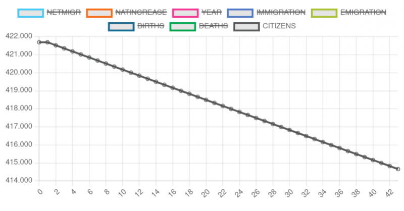
GRAPH CITIZENS
GRAPH NATINCR and NETMIGR

Here cycles 1-2 from the simulation log:
Round 1

State rules:
rworld2 applied  (Prob: 100 Rand: 40/100)
Math applied:
IMMIGRATION=CITIZENS*0.03
YEAR=YEAR+1
DEATHS=CITIZENS*0.006
BIRTHS=CITIZENS*0.0046
EMIGRATION=CITIZENS*0.029
rworld3 applied  (Prob: 0 Rand: 58/100)
Math applied:
CITIZENS=CITIZENS+NATINCREASE+NETMIGR
rworld2b applied  (Prob: 100 Rand: 6/100)
Math applied:
NATINCREASE=BIRTHS-DEATHS
NETMIGR=IMMIGRATION-EMIGRATION
Vision rules:
Current states: The number for a population in a year t+1 is the product of the population of the preceding year t enriched with the natural increase and the net migration.,The net migration is based on rates for immigration and emigrations.,The component natural increase has again two components: the rates of births and deaths.,The Main-Kinzig County exists.,A growth rate has two components: natural increase and net migration.,Based on preceding years a growth rate could be computed.,The number of citizens is known.
Current visions: The Main-Kinzig County exists.
Current values:
NETMIGR: 421.6890000000003Number
NATINCREASE: -590.3646000000001Number
YEAR: 2021Number
IMMIGRATION: 12650.67Amount
EMIGRATION: 12228.981Amount
BIRTHS: 1939.7694Amount
DEATHS: 2530.134Amount
CITIZENS: 421689Amount

50.00 percent of your vision was achieved by reaching the following states:
The Main-Kinzig County exists.,
And the following math visions:
None

Round 2

State rules:
rworld3 applied  (Prob: 0 Rand: 95/100)
Math applied:
CITIZENS=CITIZENS+NATINCREASE+NETMIGR
rworld2 applied  (Prob: 100 Rand: 22/100)
Math applied:
IMMIGRATION=CITIZENS*0.03
YEAR=YEAR+1
DEATHS=CITIZENS*0.006
BIRTHS=CITIZENS*0.0046
EMIGRATION=CITIZENS*0.029
rworld2b applied  (Prob: 100 Rand: 32/100)
Math applied:
NATINCREASE=BIRTHS-DEATHS
NETMIGR=IMMIGRATION-EMIGRATION
Vision rules:
Current states: The number for a population in a year t+1 is the product of the population of the preceding year t enriched with the natural increase and the net migration.,The net migration is based on rates for immigration and emigrations.,The component natural increase has again two components: the rates of births and deaths.,The Main-Kinzig County exists.,A growth rate has two components: natural increase and net migration.,Based on preceding years a growth rate could be computed.,The number of citizens is known.
Current visions: The Main-Kinzig County exists.
Current values:
NETMIGR: 421.5203243999986Number
NATINCREASE: -590.1284541600003Number
YEAR: 2022Number
IMMIGRATION: 12645.609732Amount
EMIGRATION: 12224.089407600002Amount
BIRTHS: 1938.9934922400003Amount
DEATHS: 2529.1219464000005Amount
CITIZENS: 421520.32440000004Amount

50.00 percent of your vision was achieved by reaching the following states:
The Main-Kinzig County exists.,
And the following math visions:
None
And here the the cycles 20-21 showing 100% success
Round 20

State rules:
rworld2b applied  (Prob: 100 Rand: 78/100)
Math applied:
NATINCREASE=BIRTHS-DEATHS
NETMIGR=IMMIGRATION-EMIGRATION
rworld3 applied  (Prob: 0 Rand: 90/100)
Math applied:
CITIZENS=CITIZENS+NATINCREASE+NETMIGR
rworld2 applied  (Prob: 100 Rand: 20/100)
Math applied:
IMMIGRATION=CITIZENS*0.03
YEAR=YEAR+1
DEATHS=CITIZENS*0.006
BIRTHS=CITIZENS*0.0046
EMIGRATION=CITIZENS*0.029
Vision rules:
Current states: The number for a population in a year t+1 is the product of the population of the preceding year t enriched with the natural increase and the net migration.,The net migration is based on rates for immigration and emigrations.,The component natural increase has again two components: the rates of births and deaths.,The Main-Kinzig County exists.,A growth rate has two components: natural increase and net migration.,Based on preceding years a growth rate could be computed.,The number of citizens is known.
Current visions: The Main-Kinzig County exists.
Current values:
NETMIGR: 418.83020290706736Number
NATINCREASE: -586.3622840698965Number
YEAR: 2040Number
IMMIGRATION: 12554.852151152843Amount
EMIGRATION: 12136.35707944775Amount
BIRTHS: 1925.077329843436Amount
DEATHS: 2510.9704302305686Amount
CITIZENS: 418495.0717050948Amount

50.00 percent of your vision was achieved by reaching the following states:
The Main-Kinzig County exists.,
And the following math visions:
None

Round 21

State rules:
rworld2 applied  (Prob: 100 Rand: 16/100)
Math applied:
IMMIGRATION=CITIZENS*0.03
YEAR=YEAR+1
DEATHS=CITIZENS*0.006
BIRTHS=CITIZENS*0.0046
EMIGRATION=CITIZENS*0.029
rworld2b applied  (Prob: 100 Rand: 28/100)
Math applied:
NATINCREASE=BIRTHS-DEATHS
NETMIGR=IMMIGRATION-EMIGRATION
rworld3 applied  (Prob: 0 Rand: 41/100)
Math applied:
CITIZENS=CITIZENS+NATINCREASE+NETMIGR
Vision rules:
Current states: The number for a population in a year t+1 is the product of the population of the preceding year t enriched with the natural increase and the net migration.,The net migration is based on rates for immigration and emigrations.,The component natural increase has again two components: the rates of births and deaths.,The Main-Kinzig County exists.,A growth rate has two components: natural increase and net migration.,Based on preceding years a growth rate could be computed.,The number of citizens is known.
Current visions: The Main-Kinzig County exists.
Current values:
NETMIGR: 418.49507170509423Number
NATINCREASE: -585.8931003871326Number
YEAR: 2041Number
IMMIGRATION: 12554.852151152843Amount
EMIGRATION: 12136.35707944775Amount
BIRTHS: 1925.077329843436Amount
DEATHS: 2510.9704302305686Amount
CITIZENS: 418327.6736764127Amount

100.00 percent of your vision was achieved by reaching the following states:
The Main-Kinzig County exists.,
And the following math visions:
YEAR>2040,
Special Comments to the Software
As mentioned in the beginning the version of the software used here is not yet the final one. We are still in an ‘experimental phase’. A feature we detected dealing with this simulation is that the simulator takes all ‘elements’ of the ‘effect part’ of a rules as ‘equal’, not applying some order for the execution. In the case of math expressions which have ‘internally’ some ‘logical order’ in the sense, that an expression A presupposes an expression B to be computed ‘before’ the expression A has to be computed (which is in this simulation clearly the case), one can handle this only if one locates all math expressions which belong to ‘the same logical level’ into a separate rule. We have to have a look to this. In such a case ‘theory’ is interacting with ‘implementation details’ which follow a quite different logic.
COMMENTS
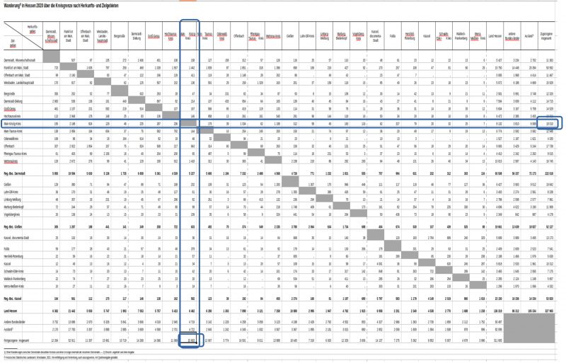
[1] Matrix of the Immigration and Emigration of citizens between the different cities and counties of the state of Hessen in 2020, Hess.Statistisches Landesamt: https://statistik.hessen.de/zahlen-fakten/bevoelkerung-gebiet-haushalte-familien/bevoelkerung/tabellen
[2] Demographic Changes between 1.January 2021 and 1.June 2021 for the MKK county, in: https://statistik.hessen.de/sites/statistik.hessen.de/files/AI2_AII_AIII_AV_21-1hj.pdf. p.7

[3] Demographic Forecast for the years 2040, Hess.Statistisches Landesamt: https://statistik.hessen.de/zahlen-fakten/bevoelkerung-gebiet-haushalte-familien/bevoelkerung/tabellen
[4] In the first paper of the small booklet from Karl Popper, „A World of Propensities“, Thoemmes Press, Bristol, (1990, repr. 1995), he develops the idea of associating an observable phenomenon with some part of the real world which has to be assumed as necessary environment for a phenomenon to be able to appear. And this presupposed empirical environment is always a complex cluster of different empirical factors interacting with each other and thereby are ‘causing’ phenomena which are not traceable to only one factor in a deterministic way but to ‘many’. ‘Chance’ is therefore a ‘product’ of reality not an isolated single event.