eJournal: uffmm.org
ISSN 2567-6458, 12.March 22 – 16.March 2022, 11:20 h
Email: info@uffmm.org
Author: Gerd Doeben-Henisch
Email: gerd@doeben-henisch.de
BLOG-CONTEXT
This post is part of the Philosophy of Science theme which is part of the uffmm blog.
PREFACE
In a preceding post I have outline the concept of an empirical theory based on a text from Popper 1971. In his article Popper points to a minimal structure of what he is calling an empirical theory. A closer investigation of his texts reveals many questions which should be clarified for a more concrete application of his concept of an empirical theory.
In this post it will be attempted to elaborate the concept of an empirical theory more concretely from a theoretical point of view as well as from an application point of view.
A Minimal Concept of an Empirical Theory
Empirical Basis
As starting point as well as a reference for testing does Popper assume an ’empirical basis’. The question arises what this means.
In the texts examined so far from Popper this is not well described. Thus in this text some ‘assumptions/ hypotheses’ will be formulated to describe some framework which should be able to ‘explain’ what an empirical basis is and how it works.
Experts
Those, who usually are building theories, are scientists, are experts. For a general concept of an ’empirical theory’ it is assumed here that every citizen is a ‘natural expert’.
Environment
Natural experts are living in ‘natural environments’ as part of the planet earth, as part of the solar system, as part of the whole universe.
Language
Experts ‘cooperate’ by using some ‘common language’. Here the ‘English language’ is used; many hundreds of other languages are possible.
Shared Goal (Changes, Time, Measuring, Successive States)
For cooperation it is necessary to have a ‘shared goal’. A ‘goal’ is an ‘idea’ about a possible state in the ‘future’ which is ‘somehow different’ to the given actual situation. Such a future state can be approached by some ‘process’, a series of possible ‘states’, which usually are characterized by ‘changes’ manifested by ‘differences’ between successive states. The concept of a ‘process’, a ‘sequence of states’, implies some concept of ‘time’. And time needs a concept of ‘measuring time’. ‘Measuring’ means basically to ‘compare something to be measured’ (the target) with ‘some given standard’ (the measuring unit). Thus to measure the height of a body one can compare it with some object called a ‘meter’ and then one states that the target (the height of the body) is 1,8 times as large as the given standard (the meter object). In case of time it was during many thousand years customary to use the ‘cycles of the sun’ to define the concept (‘unit’) of a ‘day’ and a ‘night’. Based on this one could ‘count’ the days as one day, two days, etc. and one could introduce further units like a ‘week’ by defining ‘One week compares to seven days’, or ‘one month compares to 30 days’, etc. This reveals that one needs some more concepts like ‘counting’, and associated with this implicitly then the concept of a ‘number’ (like ‘1’, ‘2’, …, ’12’, …) . Later the measuring of time has been delegated to ‘time machines’ (called ‘clocks’) producing mechanically ‘time units’ and then one could be ‘more precise’. But having more than one clock generates the need for ‘synchronizing’ different clocks at different locations. This challenge continues until today. Having a time machine called ‘clock’ one can define a ‘state’ only by relating the state to an ‘agreed time window’ = (t1,t2), which allows the description of states in a successive timely order: the state in the time-window (t1,t2) is ‘before’ the time-window (t2,t3). Then one can try to describe the properties of a given natural environment correlated with a certain time-window, e.g. saying that the ‘observed’ height of a body in time-window w1 was 1.8 m, in a later time window w6 the height was still 1.8 m. In this case no changes could be observed. If one would have observed at w6 1.9 m, then a difference is occurring by comparing two successive states.
Example: A County
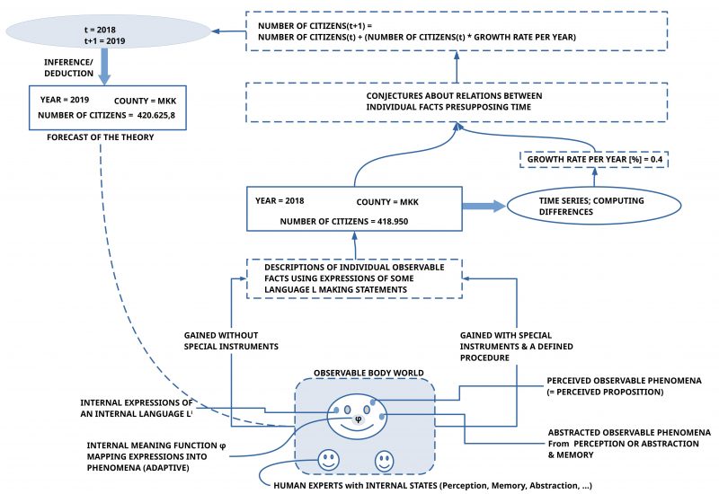
Here we will assume as an example for a natural environment a ‘county’ in Germany called ‘Main-Kinzig Kreis’ (‘Kreis’ = ‘county’), abbreviated ‘MKK’. We are interested in the ‘number of citizens’ which are living in this county during a certain time-window, here the year 2018 = (1.January 2018, 31.December 2018). According to the statistical office of the state of Hessen, to which the MKK county belongs, the number of citizens in the MKK during 2018 was ‘418.950’.(cf. [2])
Observing the Number of Citizens
One can ask in which sense the number ‘418.950’ can be understood as an ‘observation statement’? If we understand ‘observation’ as the everyday expression for ‘measuring’, then we are looking for a ‘procedure’ which allows us to ‘produce’ this number ‘418.950’ associated with the unit ‘number of citizens during a year’. As everybody can immediately realize no single person can simply observe all citizens of that county. To ‘count’ all citizens in the county one had to ‘travel’ to all places in the county where citizens are living and count every person. Such a travelling would need some time. This can easily need more than 40 years working 24 hours a day. Thus, this procedure would not work. A different approach could be to find citizens in every of the 24 cities in the MKK [1] to help in this counting-procedure. To manage this and enable some ‘quality’ for the counting, this could perhaps work. An interesting experiment. Here we ‘believe’ in the number of citizens delivered by the statistical office of the state of Hessen [2], but keeping some reservation for the question how ‘good’ this number really is. Thus our ‘observation statement’ would be: “In the year 2018 418.950 citizens have been counted in the MKK (according to the information of the statistical office of the state of Hessen)” This observation statement lacks a complete account of the procedure, how this counting really happened.
Concrete and Abstract Words
There are interesting details in this observation statement. In this observation statement we notice words like ‘citizen’ and ‘MKK’. To talk about ‘citizens’ is not a talk about some objects in the direct environment. What we can directly observe are concrete bodies which we have learned to ‘classify’ as ‘humans’, enriched for example with ‘properties’ like ‘man’, ‘woman’, ‘child’, ‘elderly person’, neighbor’ and the like. Bu to classify someone as a ‘citizen’ deserves knowledge about some official procedure of ‘registering as a citizen’ at a municipal administration recorded in some certified document. Thus the word ‘citizen’ has a ‘meaning’ which needs some ‘concrete procedure to get the needed information’. Thus ‘citizen’ is not a ‘simple word’ but a ‘more abstract word’ with regard to the associated meaning. The same holds for the word ‘MKK’ short for ‘Main-Kinzig Kreis’. At a first glance ‘MKK’ appears as a ‘name’ for some entity. But this entity cannot directly be observed too. One component of the ‘meaning’ of the name ‘MKK’ is a ‘real geographical region’, whose exact geographic extensions have been ‘measured’ by official institutions marked in an ‘official map’ of the state of Hessen. This region is associated with an official document of the state of Hessen telling, that this geographical region has to be understood s a ‘county’ with the name MKK. There exist more official documents defining what is meant with the word ‘county’. Thus the word ‘MKK’ has a rather complex meaning which to understand and to check, whether everything is ‘true’, isn’t easy. The author of this post is living in the MKK and he would not be able to tell all the details of the complete meaning of the name ‘MKK’.
First Lessons Learned
Thus one can learn from these first considerations, that we as citizens are living in a natural environment where we are using observation statements which are using words with potentially rather complex meanings, which to ‘check’ deserves some serious amount of clarification.
Conjectures – Hypotheses
Changes
The above text shows that ‘observations as such’ show nothing of interest. Different numbers of citizens in different years have no ‘message’. But as soon as one arranges the years in a ‘time line’ according to some ‘time model’ the scene is changing: if the numbers of two consecutive years are ‘different’ then this ‘difference in numbers’ can be interpreted as a ‘change’ in the environment, but only if one ‘assumes’ that the observed phenomena (the number of counted citizens) are associated with some real entities (the citizens) whose ‘quantity’ is ‘represented’ in these numbers.[5]
And again, the ‘difference between consecutive numbers’ in a time line cannot be observed or measured directly. It is a ‘second order property’ derived from given measurements in time. Such a 2nd order property presupposes a relationship between different observations: they ‘show up’ in the expressions (here numbers), but they are connected back in the light of the agreed ‘meaning’ to some ‘real entities’ with the property ‘overall quantity’ which can change in the ‘real setting’ of these real entities called ‘citizens’.
In the example of the MKK the statistical office of the state of Hessen computed a difference between two consecutive years which has been represented as a ‘growth factor’ of 0,4%. This means that the number of citizens in the year 2018 will increase until the year 2019 as follows: number-citizens(2019) = number-citizens(2018) + (number of citizens(2018) * growth-factor). This means number-citizens(2019) =418.950 + (418.950 * 0.004) = 418.950 + 1.675,8 = 420.625,8
Applying change repeatedly
If one could assume that the ‘growth rate’ would stay constant through the time then one could apply the growth rate again and again onto the actual number of citizens in the MKK every year. This would yield the following simple table:
| Year | Number | Growth Rate |
| 2018 | 418.950,00 | ,0040 |
| 2019 | 420.625,80 | |
| 2020 | 422.308,30 | |
| 2021 | 423.997,54 | |
| 2022 | 425.693,53 | |
| 2023 | 427.396,30 |
As we know from reality an assumption of a fixed growth rate for complex dynamic systems is not very probable.
Theory
Continuing the previous considerations one has to ask the question, how the layout of a ‘complete empirical theory’ would look like?
As I commented in the preceding post about Popper’s 1971 article about ‘objective knowledge’ there exists today no one single accepted framework for a formalized empirical theory. Therefore I will stay here with a ‘bottom-up’ approach using elements taken from everyday reasoning.
What we have until now is the following:
- Before the beginning of a theory building process one needs a group of experts being part of a natural environment using the same language which share a common goal which they want to enable.
- The assumed natural environment is assumed from the experts as being a ‘process’ of consecutive states in time. The ‘granularity’ of the process depends from the used ‘time model’.
- As a starting point they collect a set of statements talking about those aspects of a ‘selected state’ at some time t which they are interested in.
- This set of statements describes a set of ‘observable properties’ of the selected state which is understood as a ‘subset’ of the properties of the natural environment.
- Every statement is understood by the experts as being ‘true’ in the sense, that the ‘known meaning’ of a statement has an ‘observable counterpart’ in the situation, which can be ‘confirmed’ by each expert.
- For each pair of consecutive states it holds that the set of statements of each state can be ‘equal’ or ‘can show ‘differences’.
- A ‘difference’ between sets of statements can be interpreted as pointing to a ‘change in the real environment’.[5]
- Observed differences can be described by special statements called ‘change statements’ or simply ‘rules’.
- A change statement has the format ‘IF a set of statements ST* is a subset of the statements ST of a given state S, THEN with probability p, a set of statements ST+ will be added to the actual state S and a set of statements ST- will be removed from the statements ST of a given state S. This will result in a new succeeding state S* with the representing statements ST – (ST-) + (ST+) depending from the assumed probability p.
- The list of change statements is an ‘open set’ according to the assumption, that an actual state is only a ‘subset’ of the real environment.
- Until now we have an assumed state S, an assumed goal V, and an open set of change statements X.
- Applying change statements to a given state S will generate a new state S*. Thus the application of a subset X’ of the open set of change statements X onto a given state S will here be called ‘generating a new state by a procedure’. Such a state-generating-procedure can be understood as an ‘inference’ (like in logic) oder as a ‘simulation’ (like in engineering).[6]
- To write this in a more condensed format we can introduce some signs —– S,V ⊩ ∑ X S‘ —– saying: If I have some state S and a goal V then the simulator ∑ will according to the change statements X generate a new state S’. In such a setting the newly generated state S’ can be understood as a ‘theorem’ which has been derived from the set of statements in the state S which are assumed to be ‘true’. And because the derived new state is assumed to happen in some ‘future’ ‘after’ the ‘actual state S’ this derived state can also be understood as a ‘forecast’.
- Because the experts can change all the time all parts ‘at will’ such a ‘natural empirical theory’ is an ‘open entity’ living in an ongoing ‘communication process’.
Second Lessons Learned
It is interestingly to know that from the set of statements in state S, which are assumed to be empirically true, together with some change statements X, whose proposed changes are also assumed to be ‘true’, and which have some probability P in the domain [0,1], one can forecast a set of statements in the state S* which shall be true, with a certainty being dependent from the preceding probability P and the overall uncertainty of the whole natural environment.
Confirmation – Non-Confirmation
A Theory with Forecasts
Having reached the formulation of an ordinary empirical theory T with the ingredients <S,V,X,⊩ ∑> and the derivation concept S,V ⊩ ∑ X S‘ it is possible to generate theorems as forecasts. A forecast here is not a single statement st* but a whole state S* consisting of a finite set of statements ST* which ‘designate’ according to the ‘agreed meaning’ a set of ‘intended properties’ which need a set of ‘occurring empirical properties’ which can be observed by the experts. These observations are usually associated with ‘agreed procedures of measurement’, which generate as results ‘observation statements’/ ‘measurement statements’.
Within Time
Experts which are cooperating by ‘building’ an ordinary empirical theory are themselves part of a process in time. Thus making observations in the time-window (t1,t2) they have a state S describing some aspects of the world at ‘that time’ (t1,t2). When they then derive a forecast S* with their theory this forecast describes — with some probability P — a ‘possible state of the natural environment’ which is assumed to happen in the ‘future’. The precision of the predicted time when the forecasted statements in S* should happen depends from the assumptions in S.
To ‘check’ the ‘validity’ of such a forecast it is necessary that the overall natural process reaches a ‘point in time’ — or a time window — indicated by the used ‘time model’, where the ‘actual point in time’ is measured by an agreed time machine (mechanical clock). Because there is no observable time without a time machine the classification of a certain situation S* being ‘now’ at the predicted point of time depends completely from the used time machine.[7]
Given this the following can happen: According to the used theory a certain set of statements ST* is predicted to be ‘true’ — with some probability — either ‘at some time in the future’ or in the time-window (t1,t2) or at a certain point in time t*.
Validating Forecasts
If one of these cases would ‘happen’ then the experts would have the statements ST* of their forecast and a real situation in their natural environment which enables observations ‘Obs’ which are ‘translated’ into appropriate ‘observation statements’ STObs. The experts with their predicted statements ST* know a learned agreed meaning M* of their predicted statements ST* as intended-properties M* of ST*. The experts have also learned how they relate the intended meaning M* to the meaning MObs from the observation statements STobs. If the observed meaning MObs ‘agrees sufficiently well’ with the intended meaning M* then the experts would agree in a statement, that the intended meaning M* is ‘fulfilled’/ ‘satisfied’/ ‘confirmed’ by the observed meaning MObs. If not then it would stated that it is ‘not fulfilled’/ ‘not satisfied’/ ‘not confirmed’.
The ‘sufficient fulfillment’ of the intended meaning M* of a set of statements ST* is usually translated in a statement like “The statements ST* are ‘true'”. In the case of ‘no fulfillment’ it is unclear: this can be interpreted as ‘being false’ or as ‘being unclear’: No clear case of ‘being true’ and no clear case of ‘being false’.
Forecasting the Number of Citizens
In the used simple example we have the MKK county with an observed number of citizens in 2018 with 418950. The simple theory used a change statement with a growth factor of 0.4% per year. This resulted in the forecast with the number 420.625 citizens for the year 2019.
If the newly counting of the number of citizens in the years 2019 would yield 420.625, then there would be a perfect match, which could be interpreted as a ‘confirmation’ saying that the forecasted statement and the observed statement are ‘equal’ and therefore the theory seems to match the natural environment through the time. One could even say that the theory is ‘true for the observed time’. Nothing would follow from this for the unknown future. Thus the ‘truth’ of the theory is not an ‘absolute’ truth but a truth ‘within defined limits’.
We know from experience that in the case of forecasting numbers of citizens for some region — here a county — it is usually not so clear as it has been shown in this example.
This begins with the process of counting. Because it is very expensive to count the citizens of all cities of a county this happens only about every 20 years. In between the statistical office is applying the method of ‘forecasting projection’.[9] The state statistical office collects every year ‘electronically’ the numbers of ‘birth’, ‘death’, ‘outflow’, and ‘inflow’ from the individual cities and modifies with these numbers the last real census. In the case of the state of Hessen this was the year 2011. The next census in Germany will happen May 2022.[10] For such a census the data will be collected directly from the registration offices from the cities supported by a control survey of 10% of the population.
Because there are data from the statistical office of the state of Hessen for June 2021 [8:p.9] with saying that the MKK county had 421 936 citizens at 30. June 2021 we can compare this number with the theory forecast for the year 2021 with 423 997. This shows a difference in the numbers. The theory forecast is ‘higher’ than the observed forecast. What does this mean?
Purely arithmetically the forecast is ‘wrong’. The responsible growth factor is too large. If one would ‘adjust’ it in a simplified linear way to ‘0.24%’ then the theory could get a forecast for 2021 with 421 973 (observed: 421 936), but then the forecast for 2019 would be 419 955 (instead of 420 625).
This shows at least the following aspects:
- The empirical observations as such can vary ‘a little bit’. One had to clarify which degree of ‘variance’ is due to the method of measurement and therefore this variance should be taken into account for the evaluation of a theoretical forecast.
- As mentioned by the statistical office [9] there are four ‘factors’ which influence the final number of citizens in a region: ‘birth’, ‘death’, ‘outflow’, and ‘inflow’. These factors can change in time. Under ‘normal conditions’ the birth-rate and the death-rate are rather ‘stable’, but in case of an epidemic situation or even war this can change a lot. Outflow and inflow are very dynamic depending from many factors. Thus this can influence the growth factor a lot and these factors are difficult to forecast.
Third lessons Learned
Evaluating the ‘relatedness’ of some forecast F of an empirical theory T to the observations O in a given real natural environment is not a ‘clear-cut’ case. The ‘precision’ of such a relatedness depends from many factors where each of these factors has some ‘fuzziness’. Nevertheless as experience shows it can work in a limited way. And, this ‘limited way’ is the maximum we can get. The most helpful contribution of an ‘ordinary empirical theory’ seems to be the forecast of ‘What will happen if we have a certain set of assumptions’. Using such a forecast in the process of the experts this can help to improve to get some ‘informed guesses’ for planning.
Forecast
The next post will show, how this concept of an ordinary empirical theory can be used by applying the oksimo paradigm to a concrete case. See HERE.
Comments
[1] Cities of the MKK-county: 24, see: https://www.wegweiser-kommune.de/kommunen/main-kinzig-kreis-lk
[2] Forecast for development of the number of citizens in the MMK starting with 2018, See: the https://statistik.hessen.de/zahlen-fakten/bevoelkerung-gebiet-haushalte-familien/bevoelkerung/tabellen
[3] Karl Popper, „A World of Propensities“,(1988) and „Towards an Evolutionary Theory of Knowledge“, (1989) in: Karl Popper, „A World of Propensities“, Thoemmes Press, Bristol, (1990, repr. 1995)
[4] Karl Popper, „All Life is Problem Solving“, original a lecture 1991 in German, the first tome published (in German) „Alles Leben ist Problemlösen“ (1994), then in the book „All Life is Problem Solving“, 1999, Routledge, Taylor & Francis Group, London – New York
[5] This points to the concept of ‘propensity’ which the late Popper has discussed in the papers [3] and [4].
[6] This concept of a ‘generator’ or an ‘inference’ reminds to the general concept of Popper and the main stream philosophy of a logical derivation concept where a ‘set of logical rules’ defines a ‘derivation concept’ which allows the ‘derivation/ inference’ of a statement s* as a ‘theorem’ from an assumed set of statements S assumed to be true.
[7] The clock-based time is in the real world correlated with certain constellations of the real universe, but this — as a whole — is ‘changing’!
[8] Hessisches Statistisches Landesamt, “Die Bevölkerung der hessischen
Gemeinden am 30. Juni 2021. Fortschreibungsergebnisse Basis Zensus 09. Mai 2011″, Okt. 2021, Wiesbaden, URL: https://statistik.hessen.de/sites/statistik.hessen.de/files/AI2_AII_AIII_AV_21-1hj.pdf
[9] Method of the forward projection of the statistical office of the State of Hessen: “Bevölkerung: Die Bevölkerungszahlen sind Fortschreibungsergebnisse, die auf den bei der Zensuszählung 2011
ermittelten Bevölkerungszahlen basieren. Durch Auswertung von elektronisch übermittelten Daten für Geburten und Sterbefälle durch die Standesämter, sowie der Zu- und Fortzüge der Meldebehörden, werden diese nach einer bundeseinheitlichen Fortschreibungsmethode festgestellt. Die Zuordnung der Personen zur Bevölkerung einer Gemeinde erfolgt nach dem Hauptwohnungsprinzip (Bevölkerung am Ort der alleinigen oder der Hauptwohnung).”([8:p.2]
[10] Statistical Office state of Hessen, Next census 2022: https://statistik.hessen.de/zahlen-fakten/zensus/zensus-2022/zensus-2022-kurz-erklaert
