eJournal: uffmm.org,
ISSN 2567-6458, 2-4.April 2019
Email: info@uffmm.org
Author: Gerd Doeben-Henisch
Email: gerd@doeben-henisch.de

CONTEXT

This is a possible 3rd step in the overall topic ‘Co-Learning python3′. After downloading WinPython and activating the integrated editor ‘spyder’ (see here),  one can edit another simple program dealing with population dynamics in a most simple way (see the source code below under the title ‘EXAMPLE: pop0d.py’). This program is a continuation of the program pop0.py, which has been described here.

COMMENTS

In this post I comment only on the changes between the actual program and the version before.

IMPORTS

In the new version two libraries are used:

import matplotlib.pyplot as plt # Lib for plotting
import numpy as np # Lib for math

This extends the set of possible functions by functions for plotting and some more math.

MORE INPUT DATA

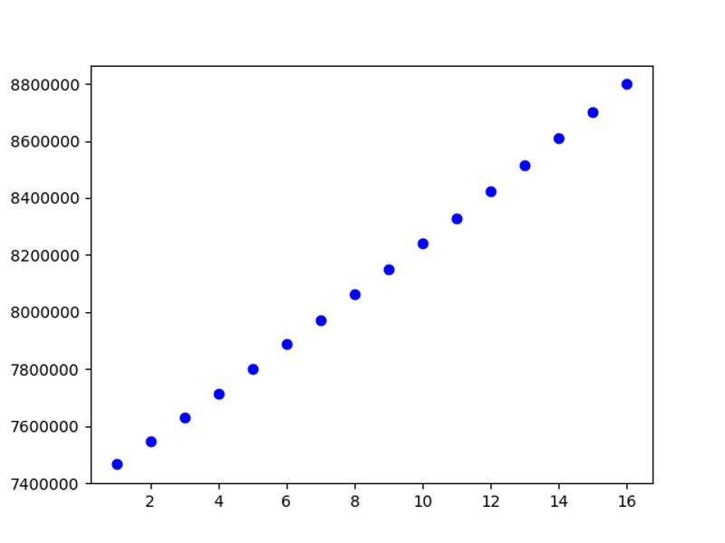
In this version one can enter a base year, thus allowing a direct relation to real year numbers in the history or the future. In the example run at the end of the program I am using the official population numbers of the UN for the world population in the years 2016 and 2017, which will hypothetically be forecasted for 15 years.

MORE GLOBAL VARIABLES

As explained in the previous version there are local variables restricted in their meaning to a certain function and global variables outside a function. In this version a datastructure called pop is introduced to store information in a sequential order. In this case the first population number given in the variable p is stored on the first position by the append operation which is part of the data structure pop.

pop = [] # storage for the pop-numbers for plotting
pop.append(p)

Later a data structure x is needed  a s a sequence of consecutive numbers starting with 1, ending with the number of entries in the pop data strucure and with as many positions as pop has entries. The number of elements in pop can be computed by applying the len() operator to pop.

x = np.linspace(1,len(pop),len(pop))

EXTENDED COMPUTATION

The computation has extended a little bit by the new line appending the actual value of p to the pop storage:

for i in range(n):
       p=pop0(p,br,dr)
      pop.append(p)

Thus the pop data structure stores every new population value in p in the sequential order of its occurence. Moreover it has been here realized a loop with the for function. The variable i is running through a sequence of values provided by the range() function. This function builts an array of numbers from 0 to n-1 and repeats therefor the call of pop0() n times.

But the most important point here is that the value of the global variable p is handed over to the function pop0(), and the local value of the variable p inside the pop0() function is again handed over by the return command to the outside of the function. Outside there is waiting the global p variable which is receiving the new value by the =-operation. In the next call of pop0() pop0() receives as new input the global variable p with the new value.

SHOWING THE RESULTS

There are now three different data show actions: (i) the list of all years with their numbers, (ii) a graphical plot of data points, and (iii) a print out of the increase of the population compared the final result with the base year.

LIST OF ALL YEARS

for i in range(n+1):
print(‘Year %5d = Citizens. %8d \n’ %(baseYear+i, pop[i]) )

Again is the for function in action ranging through the number of cycles given by the variable n. The number of the population in the different years is catched from the pop data structure by indexing the individual elements of pop by the bracket command []. pop[i] represents the i-th element of pop.

PLOTING THE POPULATION VALUES

x = np.linspace(1,len(pop),len(pop))
plt.plot(x, pop, ‘bo’)
plt.show()

The plotfunction plot of the library plt needs an arry of numbers for the x-axis given here by the x data structure, an arry of numbers for the y-axis given here by the pop-data structures, and optionally some parameter for the format of the plot symbolds. Here with ‘bo’ a black small circle. After all values are prepared will the command plt.show() make the plotted data visible.

OVERALL PERCENTAGE OF CHANGE

n1=pop[0]
n2=pop[len(pop)-1]
Increase=(n2-n1)/(n1/100)

print(“From Year %5d, until Year %5d, a change of %2.2f percent \n” % (baseYear, baseYear+n,Increase) )

Getting the base year from pop[0] and the last year from pop[len(pop)-1] one can compute the difference as the increase translated into a percentage.

REAL DATA

Although the population program is still very simple it is usefull to compute real numbers of the real world. One example are the official data of the United Nations (UN) which are collecting world wide data since their foundation 1948.

But, as a first surprise, although the UN provides lots of data from all the countries world wide, they do not systematicall a birthrate (br) or a deathrate (dr). Thus I have compiled the br and dr by inferring it from absolute population numbers from 2016 and 2017 combined with the fertility rate for 1000 people in the year 2013 averaged over all countries. This gives an estimate of 3% for the birthrate br. Using this from 2016 to 2017 this gives an ‘overshoot’ to the real numbers of 2017. I inferred from this the deathrate dr which is clearly a very week inference. Nevertheless it works for 2016 to 2017 and gives a first simple example for the upcoming years.

SOURCE CODE OF pop0d.py

pop0d.py as pop0d.pdf